

https://zh.d2l.ai/chapter_recurrent-neural-networks/sequence.html

#%matplotlib inline
import torch
from torch import nn
from d2l import torch as d2l
from API_Draw import *
T = 1000 # 总共产生1000个点
#time [0,1...,999]
time = torch.arange(1, T + 1, dtype=torch.float32)
# x = sin(timei*0.01)+高斯噪声
x = torch.sin(0.01 * time) + torch.normal(0, 0.2, (T,))
#画图
#d2l.plot(time, [x], 'time', 'x', xlim=[1, 1000], figsize=(6, 3))
#d2l.plt.show()
# 画图
#draw_pic=Animator()
#draw_pic.ShowALL_Onec(time,x) # 带噪声的
tau = 4
#T = 1000 # 总共产生1000个点
# 996 - 4 == 0
features = torch.zeros((T - tau, tau))
#features = torch.zeros((2, 3)) # 2行 3列
#print(features)
'''
tensor([[0., 0., 0.],
[0., 0., 0.]])
'''
for i in range(tau):
#print("features:",i,", x:",i,T - tau + i)
features[:, i] = x[i: T - tau + i]
'''
features: 0列 , x: 0 996
features: 1列 , x: 1 997
features: 2列 , x: 2 998
features: 3列 , x: 3 999
结果
features 有1000(总数)-4(步长)个样本 每个样本有4个连续序列
features 0-3行
0 1 2 3(列)
features 0行 x0 x1 x2 x3
features 1行 x1 x2 x3 x4
。。。
features 996行 x996 x997 x998 x999
'''
# labels torch.Size([996, 1]) --> x[4-1000] 拉伸一维度
labels = x[tau:].reshape((-1, 1))
print(labels.shape)
#torch.Size([996, 1])
batch_size, n_train = 16, 600
# 仅使用前600个“特征-标签”对进行训练
'''
features[:n_train] 取出前600 作为
features: 0 , x: 0 -600 (996)
features: 1 , x: 1 -601 (997)
features: 2 , x: 2 -602 (998)
features: 3 , x: 3 -603 (999)
'''
#n_train=20
print(features[:n_train]) # 取出前 600行(共996行)*4列 作为训练数据
train_iter = d2l.load_array((features[:n_train], labels[:n_train]),
batch_size, is_train=True)
# 初始化网络权重的函数
def init_weights(m):
if type(m) == nn.Linear:
nn.init.xavier_uniform_(m.weight)
# 一个简单的多层感知机
# #一个拥有两个全连接层的多层感知机,ReLU激活函数和平方损失。
# 样本输入位 4个序列预测一个 输入4
def get_net():
net = nn.Sequential(nn.Linear(4, 10),
nn.ReLU(),
nn.Linear(10, 1))
net.apply(init_weights)
return net
# 平方损失。注意:MSELoss计算平方误差时不带系数1/2
loss = nn.MSELoss(reduction='none')
def train(net, train_iter, loss, epochs, lr):
trainer = torch.optim.Adam(net.parameters(), lr)
for epoch in range(epochs):
i=0
for X, y in train_iter: #每个批次默认取出8个样本
trainer.zero_grad()
l = loss(net(X), y)
l.sum().backward()
trainer.step()
#print("epoch 训练周次",epoch,"样本 train_iter_i",i,"\n样本X \n",X,"\n真值y \n",y,"\n预测Y\n",net(X)) #0-38
'''
样本X 4*1*N
tensor([[-1.0703, -0.9181, -0.8705, -1.2899],
[ 0.8708, 0.9502, 1.1182, 1.1485],
[ 0.9697, 0.8139, 0.7958, 0.8831],
[-0.1353, -0.1559, -0.3127, -0.4170],
[ 0.9435, 1.2145, 0.5497, 0.7347],
[ 0.8895, 0.9038, 0.9697, 0.8139],
[ 0.9038, 0.9697, 0.8139, 0.7958],
[-0.6356, -0.6913, -1.0730, -0.6599]])
真值y 1*1*N
tensor([[-1.2054],
[ 1.0709],
[ 1.2320],
[-0.7235],
[ 1.0557],
[ 0.7958],
[ 0.8831],
[-1.0967]])
预测Y 1*1*N
tensor([[-0.8696],
[ 1.0344],
[ 0.8013],
[-0.3330],
[ 0.8102],
[ 0.9025],
[ 0.8614],
[-0.7655]], grad_fn=<AddmmBackward>)
'''
i=i+1
print(f'epoch {epoch + 1}, '
f'loss: {d2l.evaluate_loss(net, train_iter, loss):f}')
net = get_net()
train(net, train_iter, loss, 5, 0.01)
#=========================================== (1) 给我最新的4个数据,预测第5个数据,每次预测值都是真实的最新的
#预测下一个时间步的能力, 也就是单步预测(one-step-ahead prediction)。
#features 0-996
'''
结果
features 有1000(总数)-4(步长)个样本 每个样本有4个连续序列
features 0-3行
0 1 2 3(列)
features 0行 x0 x1 x2 x3
features 1行 x1 x2 x3 x4
...
features 600行 x600 x601 x603 x604
...
features 996行 x996 x997 x998 x999
'''
# 使用原始数据预测 604以后的数据 肯定对
onestep_preds = net(features)
# 可视化
d2l.plot([time, time[tau:]],
[x.detach().numpy(), onestep_preds.detach().numpy()], 'time',
'x', legend=['data', '1-step preds'], xlim=[1, 1000],
figsize=(6, 3))
d2l.plt.show()
# # 画图
#draw_pic=Animator()
#draw_pic.ShowALL_Onec(time[tau:],onestep_preds.detach().numpy()) # 带噪声的
#=============================== (2) 给定前四个真值,预测出来第五个,然后 真值(2,3,4)+预测值(5)=预测第六个值 后续往复 ,依靠少量近期数据,无限制预测未开数据(天气预报)
#我们必须使用我们自己的预测(而不是原始数据)来进行多步预测。
# T=1000 个测试数据
multistep_preds = torch.zeros(T)
# n_train =600个 训练数据
# tau = 4 步长
# x[: n_train + tau] x[604 * 4 ] 前604个真实数据 后面 1000-604 都是0
'''
multistep_preds
0-604 真实数据
605-1000 0
'''
multistep_preds[: n_train + tau] = x[: n_train + tau]
# 604-1000 使用后续都是0的真实数据来预测
for i in range(n_train + tau, T):
multistep_preds[i] = net(multistep_preds[i - tau:i].reshape((1, -1)))
#multistep_preds[i - tau:i]
# 600-603 真实数据 600 601 602 603
# 601-604 真实数据 601 602 603 预测数据 604
# 。。。
# 997-1000 预测数据 997 998 999 1000
d2l.plot([time, time[tau:], time[n_train + tau:]],
[x.detach().numpy(), onestep_preds.detach().numpy(),
multistep_preds[n_train + tau:].detach().numpy()], 'time',
'x', legend=['data', '1-step preds', 'multistep preds'],
xlim=[1, 1000], figsize=(6, 3))
d2l.plt.show()
#经过几个预测步骤之后,预测的结果很快就会衰减到一个常数。
#事实是由于错误的累积
#因此误差可能会相当快地偏离真实的观测结果。
max_steps = 64
#T=1000
#tau=4
# 1000-4-64+1= 933行 , 4+64=68列 [933,68]
features = torch.zeros((T - tau - max_steps + 1, tau + max_steps))
# 列i(i<tau)是来自x的观测,其时间步从(i)到(i+T-tau-max_steps+1)
# 0-3
for i in range(tau):
features[:, i] = x[i: i + T - tau - max_steps + 1]
# 0:0+1000-4-64+1= 933
# 1:1+1000-4-64+1= 934
# 2:2+1000-4-64+1= 935
# 3:3+1000-4-64+1= 936
'''
features [i行,前4列数据] 5-68列
x0 x1 x2 x3 0
x1 x2 x3 x4 0
...
x933 x934 x935 x936 0
'''
# 列i(i>=tau)是来自(i-tau+1)步的预测,其时间步从(i)到(i+T-tau-max_steps+1)
# 4 - 64+4=68
for i in range(tau, tau + max_steps):
features[:, i] = net(features[:, i - tau:i]).reshape(-1)
print(i-tau,i,features[:, i - tau:i],features[:, i - tau:i].shape) #933, 4
'''
features[:, i - tau:i]
列操作 列操作
真值 0-3 预测 4
真值 1 2 3 预测值4 预测 5
真值 2 3 预测值4 预测值5 预测 6
真值 3 预测值4 预测值5 预测值6 预测 7
预测值4 预测值5 预测值6 预测值7 预测 8
...
63-66 预测 67
'''
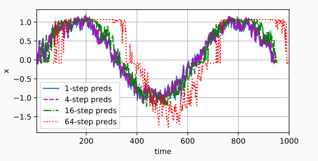
steps = (1, 4, 16, 64)
'''
time 4+1-1=4 : 1000 - 64 + 1=937 [4:937]
time 4+4-1=4 : 1000 - 64 + 4=940 [7:940]
time 4+16-1=4 : 1000 - 64 + 16=952 [19:952]
time 4+64-1=4 : 1000 - 64 + 64=1000 [67:1000]
features 4+1-1=4列 933行 真值 0-3 ==》 预测 4 列
features 4+4-1=7列 933行 真值 3 预测值4 预测值5 预测值6 ==》 预测 7列
features 4+16-1=19列 933行 预测值15 预测值16 预测值17 预测值18 ==》预测 19 列
features 4+64-1=67列 933行 预测值63 预测值64 预测值65 预测值66 ==》预测 67 列
'''
d2l.plot([time[tau + i - 1: T - max_steps + i] for i in steps],
[features[:, (tau + i - 1)].detach().numpy() for i in steps], 'time', 'x',
legend=[f'{i}-step preds' for i in steps], xlim=[5, 1000],
figsize=(6, 3))
d2l.plt.show()
API_Draw.py
### 画图 训练损失  训练精度  测试精度
import matplotlib.pyplot as plt
import threading
import time

import matplotlib.animation as animation

class Animator:
    def __init__(self):

        self.fmts=('-', 'm--', 'g-.', 'r:') #颜色 和线性

        #1 基础绘图
        #第1步:定义x和y坐标轴上的点   x坐标轴上点的数值
        self.x=[]
        #y坐标轴上点的数值
        self.train_loss=[]
        self.train_acc =[]
        self.test_acc=[]


    def add(self, x_,train_loss_,train_acc_,test_acc_ ):


        self.x.append(x_)
        self.train_loss.append(train_loss_)
        self.train_acc.append(train_acc_)
        self.test_acc.append(test_acc_)

    # 刷新最新的图像
    def ShowALL(self):


        fig, ax = plt.subplots()

        plot1=ax.plot(self.x, self.train_loss, self.fmts[0],label="train_loss")
        plot2=ax.plot(self.x, self.train_acc, self.fmts[1],label="train_acc")
        plot3=ax.plot(self.x, self.test_acc, self.fmts[2],label="test_acc")


        plt.legend(bbox_to_anchor=(1, 1),bbox_transform=plt.gcf().transFigure)# 添加图例

        plt.grid()#网格

        plt.show()


    # 画单个图
    def ShowALL_Onec(self,x,y):


        fig, ax = plt.subplots()

        plot1=ax.plot(x, y, self.fmts[0],label="--")
        #plot2=ax.plot(self.x, self.train_acc, self.fmts[1],label="train_acc")
        #plot3=ax.plot(self.x, self.test_acc, self.fmts[2],label="test_acc")


        plt.legend(bbox_to_anchor=(1, 1),bbox_transform=plt.gcf().transFigure)# 添加图例

        plt.grid()#网格

        plt.show()


import threading

import time

class MyThread(threading.Thread):

    def __init__(self,name_):

        threading.Thread.__init__(self)


        self.name_ = name_
        print("线程名字",self.name_ )

        self.is_running = 1# 控制标志位

        self.animator=Animator() # 画图类


    def run(self):

        while self.is_running:

            print("Thread is running...")

            print(self.animator.x,self.animator.train_loss)

            self.animator.ShowALL()

        print("线程停止")


    def stop(self):

        self.is_running = False


    # 创建并启动线程


# # 调用
# my_thread = MyThread("可视化训练过程")
# my_thread.setDaemon(True)#伴随主进程自动关闭
# my_thread.start()

# i=0
# while 1:
#     i=i+1
#     my_thread.animator.add(i,i-3,i-2,i-1) # 加入新数据
#     time.sleep(1)


# my_thread.stop()# 通过标志为 手动关闭

 浙公网安备 33010602011771号