一维PN结的数值模拟

问题描述

(可参考 https://www.cnblogs.com/ghzhan/articles/17031958.html)
考虑一个经典的PN结模型，掺杂浓度为 \(N_a=N_d=10^{16} cm^{-3}\), 求解其电势分布.

经典近似

一维泊松方程为:

\[\frac{d^2V}{dx^2} = -\frac{\rho}{\varepsilon} = -\frac{q(p-n+N_d-N_a)}{\varepsilon} \]

PN 结两端电势为

\[V_p = -\frac{kT}{q}ln(\frac{N_a}{n_i}), V_n = \frac{kT}{q}ln(\frac{N_d}{n_i}) \]

内建电场为:

\[V_{bi} = \frac{kT}{q}ln(\frac{N_aN_d}{n_0^2}) \]

根据耗尽层近似, 假设耗尽层宽度为 \(W\), 靠近 P 型的宽度为 \(w_p\), 靠近 N 型的宽度为 \(w_n\). 其一维泊松方程可写为:

\[\frac{d^2V}{dx^2} = \frac{qN_a}{\varepsilon} (-w_p <= x <=0)\\ = -\frac{qN_d}{\varepsilon} (0 <= x <= w_n) \]

根据边界条件 \(E(-w_p) = E(w_n) = 0, V(-w_p) = V_p, V(w_n) = V_n\), 可求得耗尽层宽度为:

\[w_n = \sqrt{\frac{2\varepsilon V_{bi}}{q(N_d+N_d^2/N_a)}}\\ w_p = \sqrt{\frac{2\varepsilon V_{bi}}{q(N_a+N_a^2/N_d)}} \]

迭代方法

事实上，耗尽层近似方法并不是一个很准确的方法。通常需要对泊松方程迭代求解来得到稳定的电势分布。下面介绍几种相关的迭代方法。

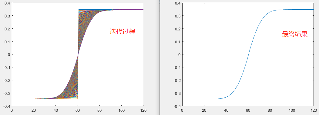
常规迭代

一维泊松方程为:

\[\frac{d^2V}{dx^2} = -\frac{\rho(V)}{\varepsilon} = -\frac{q(p-n+N_d-N_a)}{\varepsilon} \]

其中,

\[n=n_0 exp(\frac{qV}{kT}), p=n_0 exp(\frac{-qV}{kT}) \]

因此可得到:

\[\rho(V) = q[N_d-N_a - 2n_0 sinh(\frac{qV}{kT})] \]

通过有限差分, 可将 \(\frac{d^2V}{dx^2}\) 变换成矩阵形式 \(DV/a^2\), 其中 \(a\) 是差分网格密度, \(D\) 是三对角矩阵

\[D = \begin{pmatrix} -2 & 1 & \\ 1 & -2 & 1\\ &1 & -2 & 1\\ & & \ddots &\ddots &\ddots \end{pmatrix}. \]

把泊松方程写成矩阵形式:

\[DV + V_0= -\frac{qa^2}{\varepsilon}[N_d-N_a - 2n_0 sinh(\frac{qV}{kT})] \]

\(V_0\) 是与边界条件有关的常数项，这里为 \(V_0 = [V_p,0,...,0,V_n]\), 因此迭代方程为:

\[Initial - V^0 \\ V^{new} = -D^{-1}V_0 - D^{-1}\frac{qa^2}{\varepsilon}[N_d-N_a - 2n_0 sinh(\frac{qV^{old}}{kT})]\\ dV = V^{new} - V^{old}\\ V^{new} = V^{old} + 0.01*dV \]

这里的 0.01 可视情况设置。

结果如下:

Newton-Raphson

New-Raphson 方法是常用来求解非线性方程的根的方法.

\[x_{n+1}= x_n-\frac{f(x_n)}{f^{'}(x_n)}\\ f(x_n) + f^{'}(x_n) \Delta x_n = 0\\ x_{n+1} = x_n + \Delta x_n \]

因此，对于一系列的方程

\[f_i(V) = 0, i =1,2,3,...,m\\ V^{l+1}=V^{l} + \Delta V^l\\ f_i(V^{l}) + \sum_{j=1}^m\frac{\partial f_i}{\partial V_j}|_{V^l} \Delta V_j^l = 0, i=1,2,...,m. \]

对于泊松方程为

\[f(V_j) = \frac{V_{j-1}-2V_j + V_{j+1}}{a^2} + \frac{\rho(V_j)}{\varepsilon} = 0, j=1,2,...,m. \]

\(\Delta V^l\) 为

\[\frac{-\Delta V_{j-1}+2\Delta V_j-\Delta V_{j+1}}{a^2} -\frac{1}{\varepsilon}\frac{\partial\rho}{\partial V}|_{V_j} \Delta V_j = \frac{V_{j-1}-2V_j + V_{j+1}}{a^2} + \frac{\rho(V_j)}{\varepsilon} \]

上式重新写为:

\[M*\Delta V = R \]

其中:

\[M = \frac{-D}{a^2} - \frac{1}{\varepsilon}\frac{\partial\rho}{\partial V}\\ R = \frac{D}{a^2}V + \frac{\rho(V_j)}{\varepsilon} \]

对于本题中的PN结,

\[\rho(V) = q[N_d-N_a - 2n_0 sinh(\frac{qV}{kT})]\\ \frac{\partial\rho}{\partial V} = -\frac{2q^2n_0}{kT} cosh(\frac{qV}{kT}) \]

因此，根据 M 和 R 矩阵便可得到 \(\Delta V\), 再进行相应的迭代.
结果如下:

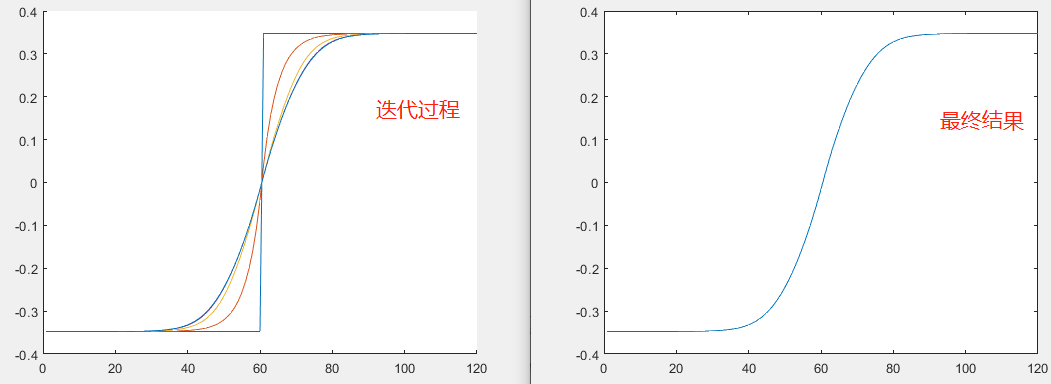
不难发现，这种迭代方法收敛很快.

Gummel 方法

"Implicit numerical schemes have to be used to solve the highly non-linear coupled Schro¨dinger–Poisson
system. Moreover, the Newton–Raphson method is not appropriate since the density does not depend
locally on the potential. Therefore, for a given potential Vn at the step n, we propose to implicit the
scheme as follows"

暂时码住. 参考文献 3.

参考文献

[1] Sunhee Lee PhD thesis. Purdue University. Appedix B. https://engineering.purdue.edu/gekcogrp/publications/theses/PhD_11_2011_Sunhee_Lee_PhD_Thesis_main.pdf
[2] R. A. Jabr, et al., Newton-Raphson solution of Poisson's equation in a pn diode. International Jounral of Electrical Engineering Eduction 44, 2007.
[3] Finley R. Shapiro, The Numerical solution of Poisson's equation in a pn Diode using a spreadsheet. IEEE TED 38, 4, 1995.
[4] E. Polizzi, N. Ben Abdallah. Subband decomposition approach for the simulation of quantum electron transport in nanostructures. Journal of Computational Physics 202, 150-180 2005.
[5] i-H. Tan, G. L. Snider, L. D. Chang, and E. L. Hu. A self‐consistent solution of Schrödinger–Poisson equations using a nonuniform mesh. Journal of Applied Physics 68, 4071–4076 (1990).
[6] https://github.com/PanosGnk/diode_model/blob/master/src/diode.m
[7] https://github.com/LaurentNevou
[8] https://github.com/SungHyunCha/NEGF_DGMOS
[9] https://github.com/giovannipizzi/SchrPoisson-2DMaterials
[10] https://ww2.mathworks.cn/matlabcentral/answers/270196-i-am-currently-writing-a-code-to-solve-poisson-equation-in-1d-for-a-pn-diode-by-iterative-newton-rap?s_tid=prof_contriblnk
[11] Arnout Beckers. Robust Simulation of Poisson’s Equation in a P-N Diode Down to 1 µK. https://arxiv.org/pdf/2212.02836v1.pdf
[12] https://lampx.tugraz.at/~hadley/psd/L6/poisson/pn_poisson_calc_live.html

附件

点击查看代码

clear all;
epsilon = 1.05*1e-12; %F/cm
q = 1.6*1e-19;% C
kT = 0.02585;% eV
n0 = 1.45*1e10; %cm^-3
theta = 1e-6;
m = 120;
Na = 1e16;
Nd = 1e16;
VP = -kT*log(Na/n0);
VN = kT*log(Nd/n0);
Na = [Na*ones(m/2,1);0*ones(m/2,1)];
Nd = [0*ones(m/2,1);Nd*ones(m/2,1)];

V=zeros(m,1);
V(1:m/2,1)=VP;    %VP has to be predefined as in (7)
V(m/2+1:m,1)=VN;  %VN has to be predefined as in (8)
D2=(2*diag(ones(1,m)))-(diag(ones(1,m-1),1))-(diag(ones(1,m-1),-1));
V0 = [VP;zeros(m-2,1);VN];
beta = q*theta*theta/epsilon;
figure;
Error = 10;
while Error > 1e-3
    hold on;
    plot(V)
    rho = Nd - Na - 2*n0*sinh(V/kT);
    V_new = inv(D2)*V0 + inv(D2)*beta*(rho);
    dv = V_new - V;
    %Error = norm(dv,2)/sqrt(m)
    Error =  max(max(abs(dv)))
    V = V + 0.1*dv;
end
figure;
plot(V)


V=zeros(m,1);
V(1:m/2,1)=VP;    %VP has to be predefined as in (7)
V(m/2+1:m,1)=VN;  %VN has to be predefined as in (8)
D2=-(2*diag(ones(1,m)))+(diag(ones(1,m-1),1))+(diag(ones(1,m-1),-1));
V0 = [VP;zeros(m-2,1);VN];
beta = q*theta*theta/epsilon;
figure;
Error = 10;
while Error > 1e-16
    hold on;
    plot(V)
    
    drho_dv = -2*n0/kT*cosh(V/kT);
    rho = Nd - Na - 2*n0*sinh(V/kT);
    
    M = -D2 - diag(beta*drho_dv);
    R = D2*V + V0 + beta*rho;
    dv = inv(M)*R;
    
    V = V + dv;
    Error = norm(dv,2)/sqrt(m);
end
figure;
plot(V)