
非线性优化一个曲线拟合(ceres/g2o)
将代码和实际理论结合起来才能更好的理解理论上是怎么实现的,参考用高博十四讲的理论加实践亲手试一下,感觉公式和代码才能结合起来。不能做到创新,至少做到了解和理解
曲线拟合问题:
考虑这样一条曲线:$y = \exp (a{x^2} + bx + c) + w$,其中a,b,c为曲线的参数,w为高斯噪声,满足$w = (0,{\sigma ^2})$,假设有N个关于x,y的观测数据点,想根据这些数据点求出曲线的参数,(误差噪声)最小二乘
\[\mathop {\min }\limits_{a,b,c} \frac{1}{2}\sum\limits_{i = 1}^N {{{\left\| {{y_i} - \exp (ax_i^2 + b{x_i} + c)} \right\|}^2}} \]
我们首先明确我们要估计的变量是a,b,c这三个系数,思路是先根据模型生成x,y的真值,然后在真值中加入高斯分布的噪声。随后使用高斯牛顿法从带噪声的数据拟合参数模型。定义误差为:${e_i} = {y_i} - \exp (ax_i^2 + b{x_i} + c)$,求取雅克比矩阵:
\[{J_i} = \left[ {\begin{array}{*{20}{c}}
{\frac{{\partial {e_i}}}{{\partial a}} = - x_i^2\exp (ax_i^2 + b{x_i} + c)}\\
{\frac{{\partial {e_i}}}{{\partial b}} = - {x_i}\exp (ax_i^2 + b{x_i} + c)}\\
{\frac{{\partial {e_i}}}{{\partial c}} = - \exp (ax_i^2 + b{x_i} + c)}
\end{array}} \right]\]
高斯牛顿法的增量方程为:
\[\left( {\sum\limits_{i = 1}^{100} {{J_i}{{({\sigma ^2})}^{ - 1}}{J_i}^T} } \right)\Delta {x_k} = \sum\limits_{i = 1}^{100} { - {J_i}{{({\sigma ^2})}^{ - 1}}{e_i}} \]
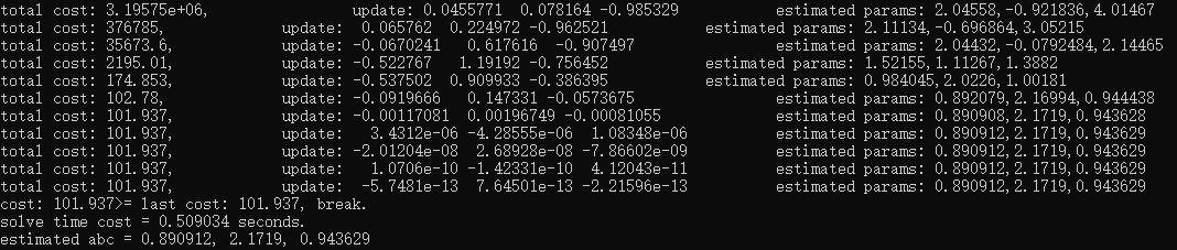
 1 #include <iostream>
 2 #include <chrono>
 3 #include <opencv2/opencv.hpp>
 4 #include <Eigen/Core>
 5 #include <Eigen/Dense>
 6 using namespace cv;
 7 using namespace std;
 8 using namespace Eigen;
 9
10 int main(int argc, char **argv) {
11     double ar = 1.0, br = 2.0, cr = 1.0;         // 真实参数值
12     double ae = 2.0, be = -1.0, ce = 5.0;        // 估计参数值,赋给一个初值,然后在这个初值的基础上进行变化量的迭代
13     int N = 100;                                 // 数据点
14     double w_sigma = 1.0;                        // 噪声Sigma值
15     double inv_sigma = 1.0 / w_sigma;           // 后面噪声1/(Sigma^2)值会用
16     cv::RNG rng;                                 // OpenCV随机数产生器
17
18     vector<double> x_data, y_data;      // 用于拟合的观测数据
19     for (int i = 0; i < N; i++) {
20         double x = i / 100.0;
21         x_data.push_back(x);
22         y_data.push_back(exp(ar * x * x + br * x + cr) + rng.gaussian(w_sigma * w_sigma));
23     }
24
25     // 开始Gauss-Newton迭代
26     int iterations = 100;    // 迭代次数
27     double cost = 0, lastCost = 0;  // 本次迭代的cost和上一次迭代的cost最小二乘值,通过此值衡量迭代是否到位,进行终止
28
29     chrono::steady_clock::time_point t1 = chrono::steady_clock::now();//计算迭代时间用
30     for (int iter = 0; iter < iterations; iter++) {
31
32         Matrix3d H = Matrix3d::Zero();             // Hessian = J^T W^{-1} J in Gauss-Newton
33         Vector3d b = Vector3d::Zero();             // bias
34         cost = 0;
35
36         for (int i = 0; i < N; i++) {
37             double xi = x_data[i], yi = y_data[i];  // 第i个数据点
38             double error = yi - exp(ae * xi * xi + be * xi + ce);
39             Vector3d J; // 雅可比矩阵
40             J[0] = -xi * xi * exp(ae * xi * xi + be * xi + ce);  // de/da
41             J[1] = -xi * exp(ae * xi * xi + be * xi + ce);  // de/db
42             J[2] = -exp(ae * xi * xi + be * xi + ce);  // de/dc
43
44             H += inv_sigma * inv_sigma * J * J.transpose();//构造Hx=b
45             b += -inv_sigma * inv_sigma * error * J;
46
47             cost += error * error;//计算最小二乘结果,看是否是最小的
48         }
49
50         // 求解线性方程 Hx=b
51         Vector3d dx = H.ldlt().solve(b);
52         if (isnan(dx[0])) {
53             cout << "result is nan!" << endl;
54             break;
55         }
56
57         if (iter > 0 && cost >= lastCost) {
58             cout << "cost: " << cost << ">= last cost: " << lastCost << ", break." << endl;
59             break;
60         }
61
62         ae += dx[0];//更新迭代量,继续迭代寻找最优值
63         be += dx[1];
64         ce += dx[2];
65
66         lastCost = cost;
67
68         cout << "total cost: " << cost << ", \t\tupdate: " << dx.transpose() <<
69             "\t\testimated params: " << ae << "," << be << "," << ce << endl;
70     }
71
72     chrono::steady_clock::time_point t2 = chrono::steady_clock::now();
73     chrono::duration<double> time_used = chrono::duration_cast<chrono::duration<double>>(t2 - t1);//给出优化用时
74     cout << "solve time cost = " << time_used.count() << " seconds. " << endl;
75
76     cout << "estimated abc = " << ae << ", " << be << ", " << ce << endl;
77     waitKey(0);
78     return 0;
79
80 }
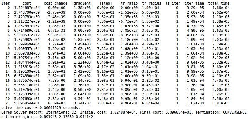
- 同样的问题用ceres库进行曲线拟合,迭代和求解过程就可以通过ceres的模板库来操作
 1 #include <iostream>
 2 #include <opencv2/core/core.hpp>
 3 #include <ceres/ceres.h>
 4 #include <chrono>
 5
 6 using namespace std;
 7
 8 // 代价函数的计算模型
 9 struct CURVE_FITTING_COST
10 {
11     CURVE_FITTING_COST ( double x, double y ) : _x ( x ), _y ( y ) {}
12     // 残差的计算
13     template <typename T>
14     bool operator() (
15         const T* const abc,     // 模型参数,有3维,也就是要要优化的参数块,
16         T* residual ) const     // 残差
17     {
18         residual[0] = T ( _y ) - ceres::exp ( abc[0]*T ( _x ) *T ( _x ) + abc[1]*T ( _x ) + abc[2] ); // y-exp(ax^2+bx+c)
19         return true;
20     }
21     const double _x, _y;    // x,y数据
22 };
23
24 int main ( int argc, char** argv )
25 {
26     double a=1.0, b=2.0, c=1.0;         // 真实参数值
27     int N=100;                          // 数据点
28     double w_sigma=1.0;                 // 噪声Sigma值
29     cv::RNG rng;                        // OpenCV随机数产生器
30     double abc[3] = {0,0,0};            // abc参数的估计值,这里初始化为0
31
32     vector<double> x_data, y_data;      // 定义观测数据
33
34     cout<<"generating data: "<<endl;
35     for ( int i=0; i<N; i++ )
36     {
37         double x = i/100.0;
38         x_data.push_back ( x );
39         y_data.push_back (
40             exp ( a*x*x + b*x + c ) + rng.gaussian ( w_sigma )
41         );
42         cout<<x_data[i]<<" "<<y_data[i]<<endl;//产生观测数据
43     }
44
45     // 构建最小二乘问题
46     ceres::Problem problem;
47     for ( int i=0; i<N; i++ )
48     {
49         problem.AddResidualBlock (     // 向问题中添加误差项
50         // 使用自动求导,模板参数:误差类型,输出维度,输入维度,维数要与前面struct中一致
51             new ceres::AutoDiffCostFunction<CURVE_FITTING_COST, 1, 3> (
52                 new CURVE_FITTING_COST ( x_data[i], y_data[i] )// 观测数据
53             ),
54             nullptr,            // 核函数,这里不使用,为空
55             abc                 // 待估计参数
56         );
57     }
58
59     // 配置求解器
60     ceres::Solver::Options options;     // 这里有很多配置项可以填
61     options.linear_solver_type = ceres::DENSE_QR;  // 增量方程如何求解
62     options.minimizer_progress_to_stdout = true;   // 输出到cout
63
64     ceres::Solver::Summary summary;                // 优化信息
65     chrono::steady_clock::time_point t1 = chrono::steady_clock::now();
66     ceres::Solve ( options, &problem, &summary );  // 开始优化
67     chrono::steady_clock::time_point t2 = chrono::steady_clock::now();
68     chrono::duration<double> time_used = chrono::duration_cast<chrono::duration<double>>( t2-t1 );
69     cout<<"solve time cost = "<<time_used.count()<<" seconds. "<<endl;
70
71     // 输出结果
72     cout<<summary.BriefReport() <<endl;
73     cout<<"estimated a,b,c = ";
74     for ( auto a:abc ) cout<<a<<" ";
75     cout<<endl;
76
77     return 0;
78 }
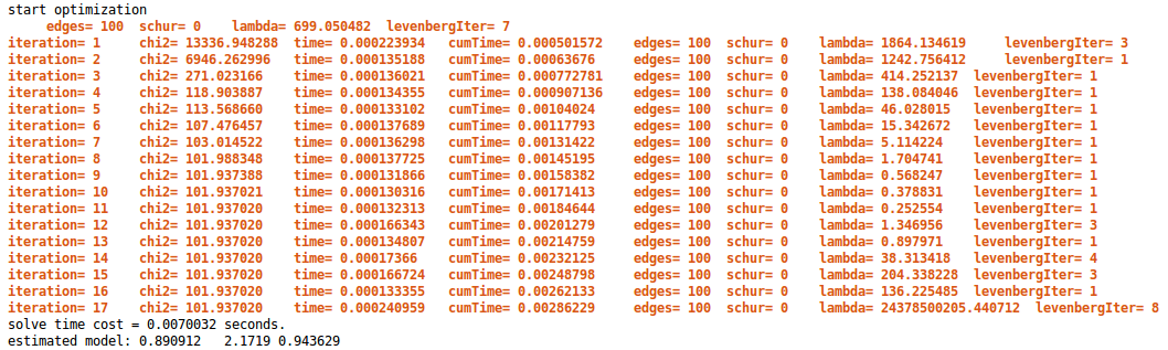
- 图优化(g2o)进行曲线拟合参照图优化系列-g2o细细看,多看几遍中间的来龙去脉
  1 #include <iostream>
  2 #include <g2o/core/base_vertex.h>
  3 #include <g2o/core/base_unary_edge.h>
  4 #include <g2o/core/block_solver.h>
  5 #include <g2o/core/optimization_algorithm_levenberg.h>
  6 #include <g2o/core/optimization_algorithm_gauss_newton.h>
  7 #include <g2o/core/optimization_algorithm_dogleg.h>
  8 #include <g2o/solvers/dense/linear_solver_dense.h>
  9 #include <Eigen/Core>
 10 #include <opencv2/core/core.hpp>
 11 #include <cmath>
 12 #include <chrono>
 13 using namespace std;
 14
 15 // 曲线模型的顶点,模板参数:优化变量维度和数据类型
 16 class CurveFittingVertex: public g2o::BaseVertex<3, Eigen::Vector3d>
 17 {
 18 public:
 19     EIGEN_MAKE_ALIGNED_OPERATOR_NEW
 20     virtual void setToOriginImpl() // 重置
 21     {
 22         _estimate << 0,0,0;
 23     }
 24
 25     virtual void oplusImpl( const double* update ) // 更新
 26     {
 27         _estimate += Eigen::Vector3d(update);
 28     }
 29     // 存盘和读盘:留空
 30     virtual bool read( istream& in ) {}
 31     virtual bool write( ostream& out ) const {}
 32 };
 33
 34 // 误差模型 模板参数:观测值维度,类型,连接顶点类型
 35 class CurveFittingEdge: public g2o::BaseUnaryEdge<1,double,CurveFittingVertex>
 36 {
 37 public:
 38     EIGEN_MAKE_ALIGNED_OPERATOR_NEW
 39     CurveFittingEdge( double x ): BaseUnaryEdge(), _x(x) {}
 40     // 计算曲线模型误差
 41     void computeError()
 42     {
 43         const CurveFittingVertex* v = static_cast<const CurveFittingVertex*> (_vertices[0]);
 44         const Eigen::Vector3d abc = v->estimate();
 45         _error(0,0) = _measurement - std::exp( abc(0,0)*_x*_x + abc(1,0)*_x + abc(2,0) ) ;
 46     }
 47     virtual bool read( istream& in ) {}
 48     virtual bool write( ostream& out ) const {}
 49 public:
 50     double _x;  // x 值, y 值为 _measurement
 51 };
 52
 53 int main( int argc, char** argv )
 54 {
 55     double a=1.0, b=2.0, c=1.0;         // 真实参数值
 56     int N=100;                          // 数据点
 57     double w_sigma=1.0;                 // 噪声Sigma值
 58     cv::RNG rng;                        // OpenCV随机数产生器
 59     double abc[3] = {0,0,0};            // abc参数的估计值
 60
 61     vector<double> x_data, y_data;      // 数据
 62
 63     cout<<"generating data: "<<endl;
 64     for ( int i=0; i<N; i++ )
 65     {
 66         double x = i/100.0;
 67         x_data.push_back ( x );
 68         y_data.push_back (
 69             exp ( a*x*x + b*x + c ) + rng.gaussian ( w_sigma )
 70         );
 71         cout<<x_data[i]<<" "<<y_data[i]<<endl;
 72     }
 73
 74     // 构建图优化,先设定g2o
 75     typedef g2o::BlockSolver< g2o::BlockSolverTraits<3,1> > Block;  // 每个误差项优化变量维度为3,误差值维度为1
 76     Block::LinearSolverType* linearSolver = new g2o::LinearSolverDense<Block::PoseMatrixType>(); // 线性方程求解器
 77     Block* solver_ptr = new Block( linearSolver );      // 矩阵块求解器
 78     // 梯度下降方法,从GN, LM, DogLeg 中选
 79     g2o::OptimizationAlgorithmLevenberg* solver = new g2o::OptimizationAlgorithmLevenberg( solver_ptr );
 80     // g2o::OptimizationAlgorithmGaussNewton* solver = new g2o::OptimizationAlgorithmGaussNewton( solver_ptr );
 81     // g2o::OptimizationAlgorithmDogleg* solver = new g2o::OptimizationAlgorithmDogleg( solver_ptr );
 82     g2o::SparseOptimizer optimizer;     // 图模型
 83     optimizer.setAlgorithm( solver );   // 设置求解器
 84     optimizer.setVerbose( true );       // 打开调试输出
 85
 86     // 往图中增加顶点
 87     CurveFittingVertex* v = new CurveFittingVertex();
 88     v->setEstimate( Eigen::Vector3d(0,0,0) );
 89     v->setId(0);
 90     optimizer.addVertex( v );
 91
 92     // 往图中增加边
 93     for ( int i=0; i<N; i++ )
 94     {
 95         CurveFittingEdge* edge = new CurveFittingEdge( x_data[i] );
 96         edge->setId(i);
 97         edge->setVertex( 0, v );                // 设置连接的顶点
 98         edge->setMeasurement( y_data[i] );      // 观测数值
 99         edge->setInformation( Eigen::Matrix<double,1,1>::Identity()*1/(w_sigma*w_sigma) ); // 信息矩阵:协方差矩阵之逆
100         optimizer.addEdge( edge );
101     }
102
103     // 执行优化
104     cout<<"start optimization"<<endl;
105     chrono::steady_clock::time_point t1 = chrono::steady_clock::now();
106     optimizer.initializeOptimization();
107     optimizer.optimize(100);
108     chrono::steady_clock::time_point t2 = chrono::steady_clock::now();
109     chrono::duration<double> time_used = chrono::duration_cast<chrono::duration<double>>( t2-t1 );
110     cout<<"solve time cost = "<<time_used.count()<<" seconds. "<<endl;
111
112     // 输出优化值
113     Eigen::Vector3d abc_estimate = v->estimate();
114     cout<<"estimated model: "<<abc_estimate.transpose()<<endl;
115
116     return 0;
117 }

 浙公网安备 33010602011771号