NumPy 入门示例系列01

参考：

https://www.cnblogs.com/emanlee/p/16025421.html

 

NumPy（Numerical Python）是Python的一种开源的数值计算扩展。这种工具可用来存储和处理大型矩阵，比Python自身的嵌套列表（nested list structure）结构要高效得多（该结构也可以用来表示矩阵（matrix）），支持大量的维度数组与矩阵运算，此外也针对数组运算提供大量的数学函数库。

 

安装 NumPy

使用NumPy之前，需要安装。

安装

pip install numpy

查看版本 

import numpy as np
print(np.__version__)

 

简单示例

示例：

import numpy as np #导入NumPy库，给一个别名np
 
x = np.arange ( 5 )  
print ( x ) # 输出 [0 1 2 3 4]

解释：

np.arange(5) 是 NumPy 库中的一个函数调用，用于生成一个从 0 开始、步长为 1、到（但不包含）5 的一维数组。

其输出结果为：  

array([0, 1, 2, 3, 4]) 

解析：

• arange 函数的基本语法是 np.arange([start=0,] stop[, step=1,], dtype=None)
• 当只传入一个参数时，该参数表示 stop（终止值），start 默认为 0，step 默认为 1
• 因此 np.arange(5) 等价于 np.arange(0, 5, 1)，生成包含 0、1、2、3、4 的数组

 

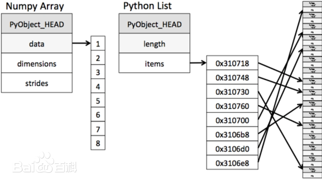
NumPy提供了一个N维数组类型 ndarray，它描述了相同类型的“items”的集合。
ndarray 跟原生python列表的区别：
从下图中可以看出ndarray在存储数据的时候，数据与数据的地址都是连续的，这样就使得批量操作数组元素时速度更快。
这是因为ndarray中的所有元素的类型都是相同的，而Python列表中的元素类型是任意的，所以ndarray在存储元素时内存可以连续，而python原生list就只能通过寻址方式找到下一个元素，这虽然也导致了在通用性能方面NumPy的ndarray不及Python原生list，但在科学计算中，NumPy的ndarray就可以省掉很多循环语句，代码使用方面比Python原生list简单得多。
NumPy内置了并行运算功能，当系统有多个核心时，做某种计算时，NumPy会自动做并行计算。
NumPy底层使用C语言编写，数组中直接存储对象，而不是存储对象指针，所以其运算效率远高于纯Python代码。

快速入门

NumPy 包的核心是 ndarray 对象。
它封装了同质数据类型的 n 维数组，为了提高性能，许多操作在编译后的代码中执行。

 

NumPy 的数组类名为ndarray 。它也有一个别名 array 。

请注意， numpy.array 与 Python 标准库中的类 array.array 不同，后者仅处理一维数组，且功能较少。
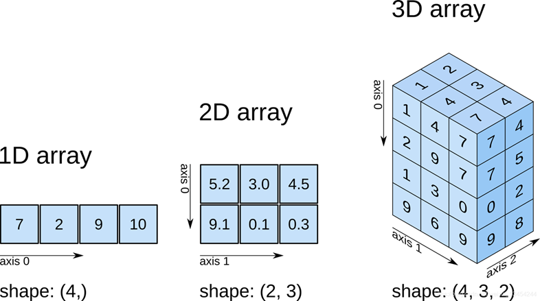
生成数组的方法（创建数组的方法）：

>>> import numpy as np

>>> one = np.array( [ 7, 2, 9, 10 ] )
>>> one.shape
(4,)

>>> two = np.array( [ [ 5.2, 3.0, 4.5 ], [ 9.1, 0.1, 0.3 ] ] )
>>> two.shape
(2, 3)

>>> three = np.array( [ [ [ 1, 1 ], [ 1, 1 ], [ 1, 1 ] ],
 [ [ 1, 1 ], [ 1, 1 ], [ 1, 1 ] ],
 [ [ 1, 1 ], [ 1, 1 ], [ 1, 1 ] ],
 [ [ 1, 1 ], [ 1, 1 ], [ 1, 1 ] ] ] )
>>> three.shape
(4, 3, 2)

  

如果array里有一个元素是字符，则所有元素都会变成string类型（数据的元素的类型必须相同）：

>>> a = np.array ( [ 0, 1, 2, 3, 'abc' ] )
>>> a
array(['0', '1', '2', '3', 'abc'], dtype='<U21')

 

The Basic 基础知识—— An Example

ndarray.dtype : the type of the elements in the array.  数组中元素类型。可用标准 Python数据类型。NumPy 还提供了自己的类型，numpy.int32、numpy.int16 和 numpy.float64。
ndarray.itemsize : the size in bytes of each element of the array. 数组中每个元素的大小（以字节为单位）。float64类型占用8个字节内存空间
ndarray.ndim : the number of axes (dimensions) of the array. 数组的轴数（维度数量）
ndarray.shape : the dimensions of the array. 数组的维度。为整数元组，表示每个维度上的大小。
ndarray.size : the total number of elements of the array.  数组元素的总数。等于shape的乘积。

 

NumPy 的数组中比较重要 ndarray 对象属性有：

属性	说明
ndarray.ndim	秩，即轴的数量或维度的数量
ndarray.shape	数组的维度，对于矩阵，n 行 m 列
ndarray.size	数组元素的总个数，相当于 .shape 中 n*m 的值
ndarray.dtype	ndarray 对象的元素类型
ndarray.itemsize	ndarray 对象中每个元素的大小，以字节为单位
ndarray.flags	ndarray 对象的内存信息
ndarray.real	ndarray元素的实部
ndarray.imag	ndarray 元素的虚部
ndarray.data	包含实际数组元素的缓冲区，由于一般通过数组的索引获取元素，所以通常不需要使用这个属性。

>>> import numpy as np
>>> a = np.arange( 15 )
>>> a
array([ 0,  1,  2,  3,  4,  5,  6,  7,  8,  9, 10, 11, 12, 13, 14])
>>> a.shape #
(15,)
>>> a.ndim #
1
>>> a.dtype.name
'int64'
>>> a.itemsize #
8
>>> a.size #
15
>>> type(a)
<class 'numpy.ndarray'>

>>> b = a.reshape( 3, 5 )
>>> b
array([[ 0,  1,  2,  3,  4],
       [ 5,  6,  7,  8,  9],
       [10, 11, 12, 13, 14]])
>>> b.shape
(3, 5)
>>> b.ndim
2
>>> b.dtype.name
'int64'
>>> b.itemsize
8
>>> b.size
15
>>> type(b)
<class 'numpy.ndarray'>

 

在 NumPy 中，a.reshape(3, 5) 是数组对象 a 的一个方法，用于将数组 a 重塑为指定形状的新数组，这里的目标形状是 3 行 5 列（即 3×5 的二维数组）。

说明：

1. 形状要求： 原数组 a 的元素总数必须与目标形状的元素总数相等（即 3×5=15），否则会报错。例如，若 a 是一个包含 15 个元素的一维数组（如 np.arange(15)），则可以成功重塑为 3×5 的二维数组。
2. 返回新数组，不改变原数组： reshape 方法不会修改原数组 a 本身，而是返回一个形状改变后的新数组。如果需要直接修改原数组，可以使用 a.shape = (3, 5)（但需注意同样要求元素总数匹配）。
3. 内存共享： 重塑后的数组与原数组通常共享同一块内存（视图，view），即修改其中一个数组的值，另一个也会随之改变（除非原数组是副本）。

The basics——Array creation 数组创建

>>> np.zeros((3, 4)) # 创建指定大小的数组，数组元素以 0 来填充
array([[0., 0., 0., 0.],
       [0., 0., 0., 0.],
       [0., 0., 0., 0.]])
>>> d = np.zeros((3, 4))
>>> d
array([[0., 0., 0., 0.],
       [0., 0., 0., 0.],
       [0., 0., 0., 0.]])

>>> e = np.ones((2, 3, 4), dtype=np.int16) # 创建指定大小的数组，数组元素以 1 来填充
>>> e
array([[[1, 1, 1, 1],
        [1, 1, 1, 1],
        [1, 1, 1, 1]],

       [[1, 1, 1, 1],
        [1, 1, 1, 1],
        [1, 1, 1, 1]]], dtype=int16)

>>> f = np.empty((2, 3)) # 2行3列的随机数组
>>> f
array([[3.44900708e-307, 4.22786102e-307, 2.78145267e-307],
       [4.00537061e-307, 2.23419104e-317, 0.00000000e+000]])

 

>>> np.arange ( 10, 30, 5 )
array([10, 15, 20, 25])
>>> np.arange ( 0, 2, 0.3 ) # 步长可以是浮点数
array([0. , 0.3, 0.6, 0.9, 1.2, 1.5, 1.8])

>>> np.linspace ( 0, 2, 9 )  # 下面有解释
array([0.,0.25,0.5,0.75,1.,1.25,1.5,1.75,2.])
>>> x = np.linspace ( 0, 2 * np.pi, 100 )
>>> f = np.sin(x)

函数arange由于浮点精度有限，通常无法预测获得的元素数量，应该使用函数 linspace

 

numpy.linspace

linspace 是‌ linear space‌ 的缩写，中文含义为‌线性等分向量‌或‌线性平分向量‌，用于将线性空间等分生成数值序列。

numpy.linspace 函数用于创建一个一维数组，数组是一个等差数列构成的，格式如下：

np.linspace(start, stop, num=50, endpoint=True, retstep=False, dtype=None)

参数说明：

参数	描述
start	序列的起始值
stop	序列的终止值，如果endpoint为true，该值包含于数列中
num	要生成的等步长的样本数量，默认为50
endpoint	该值为 true 时，数列中包含stop值，反之不包含，默认是True。
retstep	如果为 True 时，生成的数组中会显示间距，反之不显示。
dtype	ndarray 的数据类型

 

The type of the array can also be explicitly specified at creation time:
数组的类型也可以在创建时明确指定：

>>> c = np.array([[1, 2], [3, 4]], dtype=complex)
>>> c
array([[1.+0.j, 2.+0.j],
       [3.+0.j, 4.+0.j]])

 

The basics——Printing arrays 打印数组

When you print an array, NumPy displays it in a similar way to nested lists, but with the following layout:打印数组时，NumPy 以类似于嵌套列表的方式显示它，但采用以下布局：
the last axis is printed from left to right, 最后一个轴从左到右打印，
the second-to-last is printed from top to bottom, 倒数第二个从上到下打印，
the rest are also printed from top to bottom, with each slice separated from the next by an empty line. 其余部分也从上到下打印，每个切片与下一个切片之间用空行分隔。
One-dimensional arrays are then printed as rows, bidimensionals as matrices and tridimensionals as lists of matrices.  将一维数组打印为行，将二维数组打印为矩阵，将三维数组打印为矩阵列表。

>>> a = np.arange(6)
>>> a
array([0, 1, 2, 3, 4, 5])
>>> print(a)
[0 1 2 3 4 5]

>>> b = np.arange(12).reshape(4, 3)
>>> print(b)
[[ 0  1  2]
 [ 3  4  5]
 [ 6  7  8]
 [ 9 10 11]]

>>> c = np.arange(24).reshape(2, 3, 4)
>>> print(c)
[[[ 0  1  2  3]
  [ 4  5  6  7]
  [ 8  9 10 11]]

 [[12 13 14 15]
  [16 17 18 19]
  [20 21 22 23]]]

 

>>> print(np.arange(10000))
[   0    1    2 ... 9997 9998 9999]
>>> print(np.arange(10000).reshape(100, 100))
[[   0    1    2 ...   97   98   99]
 [ 100  101  102 ...  197  198  199]
 [ 200  201  202 ...  297  298  299]
 ...
 [9700 9701 9702 ... 9797 9798 9799]
 [9800 9801 9802 ... 9897 9898 9899]
 [9900 9901 9902 ... 9997 9998 9999]]

 

The basics——Basic operations 基本操作

Arithmetic operators on arrays apply elementwise. A new array is created and filled with the result. 数组上的算术运算符按元素进行操作。创建一个新数组并用结果填充。

>>> a = np.array( [ 20, 30, 40, 50 ] )
>>> b = np.arange( 4 )
>>> b
array( [ 0, 1, 2, 3 ] )
>>> c = a - b
>>> c
array( [ 20, 29, 38, 47 ] )
>>> b ** 2
array( [ 0, 1, 4, 9 ] )
>>> 10 * np.sin( a )
array( [ 9.129, -9.880,  7.451 , -2.623] )
>>> a < 35
array( [ True,  True, False, False ] )

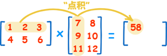
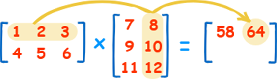
The product operator * operates elementwise in NumPy arrays. The matrix product can be performed using the @ operator or the dot function or method 乘积运算符 * 在 NumPy 数组中按元素进行运算。矩阵乘积可以使用 @ 运算符或 dot 函数或方法执行。

元素级乘法（ * 元素乘积）

• 用于一维数组或矩阵的对应元素相乘，例如a * b会计算a和b对应位置的乘积。

矩阵乘法（ @  点积）

• np.dot(a, b)计算两个矩阵的点积（对应元素相乘后求和），适用于向量或矩阵。 ‌
• np.matmul(a, b)功能与np.dot相同，但更符合线性代数标准。

 

>>> A = np.array( [ [ 1, 1 ],  [ 0, 1 ] ] )
>>> B = np.array( [ [ 2, 0 ],  [ 3, 4 ] ] )
>>> A * B
array( [ [ 2, 0 ],
       [ 0, 4 ] ] )
>>> A @ B
array( [ [ 5, 4 ],
       [ 3, 4 ] ] )
>>> A.dot ( B )
array( [ [ 5, 4 ],
       [ 3, 4 ] ] )

 

 

点积（线性代数中的矩阵乘法），如下图所示： 

 

 

The basics——Basic operations 基本操作

Some operations, such as += and *=, act in place to modify an existing array rather than create a new one. 某些操作（例如 += 和 *= ）会修改现有数组，而不是创建新数组。

>>> a = np.ones((2, 5), dtype=int)
>>> a
array( [ [ 1, 1, 1, 1, 1 ],
       [ 1, 1, 1, 1, 1 ] ] )
>>> b = np.linspace(0,1,10).reshape(2,5)
>>> b
array( [ [ 0.        , 0.11111111, 0.22222222, 0.33333333, 0.44444444 ],
       [ 0.55555556, 0.66666667, 0.77777778, 0.88888889, 1.        ] ] )

>>> a *= 3
>>> a
array( [ [ 3, 3, 3, 3, 3 ],
       [ 3, 3, 3, 3, 3 ] ] )
>>> b += a
>>> b
array( [ [ 3.        , 3.11111111, 3.22222222, 3.33333333, 3.44444444 ],
       [ 3.55555556, 3.66666667, 3.77777778, 3.88888889, 4.        ] ] )

>>> a += b
Traceback (most recent call last):
  File "<python-input-96>", line 1, in <module>
    a += b
numpy._core._exceptions._UFuncOutputCastingError: Cannot cast ufunc 'add' output from dtype('float64') to dtype('int64') with casting rule 'same_kind'

 

The basics——Basic operations 基本操作

When operating with arrays of different types, the type of the resulting array corresponds to the more general or precise one (a behavior known as upcasting).
当操作不同类型的数组时，结果数组的类型对应于更通用或更精确的类型（这种行为称为向上转型）。

>>> a = np.ones(3, dtype=np.int32)
>>> a
array([1, 1, 1], dtype=int32)
>>> b = np.linspace(0, np.pi, 3)
>>> b
array([0.        , 1.57079633, 3.14159265])
>>> b.dtype.name
'float64'
>>> c = a + b
>>> c
array([1.        , 2.57079633, 4.14159265])
>>> c.dtype.name
'float64'
>>> d = np.exp(c * 1j )
>>> d
array([ 0.54+0.84j, -0.84+0.54j, -0.54-0.84j])
>>> d.dtype.name
'complex128'

Many unary operations are implemented as methods of the ndarray class.许多一元运算都是作为 ndarray 类的方法实现的。

>>> a = np.arange(5)
>>> a
array([0, 1, 2, 3, 4])

>>> a.sum()
np.int64(10)
>>> a.min()
np.int64(0)
>>> a.max()
np.int64(4)

 

By specifying the axis parameter you can apply an operation along the specified axis of an array 通过指定 axis 参数，您可以沿数组的指定轴应用操作

>>> b = np.arange(6).reshape(2,3)
>>> b
array([[0, 1, 2],
       [3, 4, 5]])

>>> b.sum(axis=0)
array([3, 5, 7])
>>> b.sum(axis=1)
array([ 3, 12])

 

The basics——Universal functions通用函数

NumPy provides familiar mathematical functions such as sin, cos, and exp. In NumPy, these are called “universal functions” (ufunc). Within NumPy, these functions operate elementwise on an array, producing an array as output.
-- NumPy 提供了一些常见的数学函数，例如 sin、cos 和 exp。在 NumPy 中，这些函数被称为“通用函数”（ ufunc ）。在 NumPy 中，这些函数对数组进行逐元素运算，并生成一个数组作为输出。

>>> B = np.arange(3)
>>> B
array([0, 1, 2])

>>> np.exp(B)
array([1.        , 2.71828183, 7.3890561 ])
>>> np.sqrt(B)
array([0.        , 1.        , 1.41421356])

>>> C = np.array ( [ 2.0, -1.0, 4.0 ] )
>>> np.add ( B, C )
array([2., 0., 6.])

 

The basics——Indexing, slicing and iterating索引、切片和迭代

One-dimensional arrays can be indexed, sliced and iterated over, much like lists and other Python sequences一维数组可被索引/切片/迭代，就像list 和其他 Python 序列一样。

示例：

>>> a = np.arange(10)**3
>>> a
array([  0,   1,   8,  27,  64, 125, 216, 343, 512, 729])

>>> a [ 2 ]
np.int64(8)
>>> a [ 2 : 5 ]
array([ 8, 27, 64])

>>> a [ 0 : 6 : 2 ] = 1000
>>> a
array([1000,    1, 1000,   27, 1000,  125,  216,  343,  512,  729])

>>> a [ : : -1 ]
array([ 729,  512,  343,  216,  125, 1000,   27, 1000,    1, 1000])

数组切片 a[0 : 6 : 2]

这是对数组 a 的切片操作，语法为 a[start:stop:step]，表示： 

• start=0：从索引 0 开始（包含该元素）。
• stop=6：到索引 6 结束（不包含该元素）。
• step=2：步长为 2，即每隔 1 个元素取一个。
  因此，切片选取的索引为 0、2、4（从 0 开始，每次加 2，直到小于 6），对应的值为：

  array([0, 8, 64])

Shape manipulation 维度/形状的操作

Changing the shape of an array 改变数组的形状
An array has a shape given by the number of elements along each axis
-- 数组的形状由沿每个轴的元素数量决定

>>> a = np.arange( 15 )
>>> a
array( [ 0,  1,  2,  3,  4,  5,  6,  7,  8,  9, 10, 11, 12, 13, 14 ] )
>>> a.shape
(15,)
>>> b = a.reshape( 3, 5 )
>>> b
array( [ [ 0,  1,  2,  3,  4 ],
       [ 5,  6,  7,  8,  9 ],
       [10, 11, 12, 13, 14 ] ] )
>>> b.shape
(3, 5)
>>> c = b.ravel( ) # 英[ˈrævl] 作及物动词时译为“解开（线圈等）；弄清”，作不及物动词时译为“使更复杂”
>>> c
array( [ 0,  1,  2,  3,  4,  5,  6,  7,  8,  9, 10, 11, 12, 13, 14] )
>>> e = b.T # 转置
>>> c.shape
(15,)
>>> e
array( [ [ 0,  5, 10 ],
       [ 1,  6, 11 ],
       [ 2,  7, 12 ],
       [ 3,  8, 13 ],
       [ 4,  9, 14 ] ] )
>>> e.shape
(5, 3)

• ravel() 是 NumPy 数组的一个方法，用于将任意维度的数组展平为一维数组（即去除所有维度，只保留一行元素）。
• 对于本身已是一维的数组（如 b），ravel() 会返回一个与原数组相同的一维数组（但通常是原数组的视图，共享内存）。

Stacking together different arrays 将不同的数组堆叠在一起
Several arrays can be stacked together along different axes:
-- 可以沿不同的轴将多个数组堆叠在一起

>>> a = np.arange( 1, 5, ).reshape( 2, 2 )
>>> a
array( [ [ 1, 2 ],
       [ 3, 4 ] ] )
>>> b = np.arange( 11, 15, ).reshape( 2, 2 )
>>> b
array( [ [ 11, 12 ],
       [ 13, 14 ] ] )

>>> c = np.vstack( ( a, b ) ) # Vertical Stack（垂直堆叠） 英文读作/viː stæk/， 直译为"V堆叠"或"垂直堆叠函数"
>>> c
array( [ [ 1,  2 ],
       [ 3,  4 ],
       [11, 12 ],
       [13, 14 ] ] )
>>> d = np.hstack ( ( a, b ) ) # “H”代表“horizontal”（水平方向），因此中文习惯称为‌水平堆叠函数‌，用于将多个数组横向排列组合。‌‌
>>> d
array( [ [ 1,  2, 11, 12 ],
       [ 3,  4, 13, 14 ] ] )

np.vstack((a, b)) 是 NumPy 中的一个函数，用于将两个数组 垂直堆叠（vertical stack）[ˈvɜːtɪkl]，即按行拼接，将数组 b 堆叠在数组 a 的下方，形成一个新的数组。

两个数组 a 和 b 必须满足 列数相同（即第二维的长度一致），否则会报错。

 

np.hstack((a, b)) 是 NumPy 中的函数，用于将两个数组 水平堆叠（horizontal stack）[ˌhɒrɪˈzɒntl]，即按列拼接，将数组 b 拼接在数组 a 的右侧，形成一个新的数组。

两个数组 a 和 b 必须满足 行数相同（即第一维的长度一致），否则会报错。

Splitting one array into several smaller ones将一个数组拆分成几个较小的数组
使用 hsplit 沿水平轴拆分数组，方法是指定要返回的相同形状数组的数量，或者指定应在之后进行划分的列。

使用vsplit 沿垂直轴分割， array_split 允许指定沿哪个轴分割。

>>> a = np.arange( 18 ).reshape( 3, 6 )
>>> a
array( [ [ 0,  1,  2,  3,  4,  5 ],
       [ 6,  7,  8,  9, 10, 11 ],
       [12, 13, 14, 15, 16, 17 ] ] )

>>> b, c, d = np.hsplit( a, 3 )
>>> b
array( [ [ 0,  1 ],
       [ 6,  7 ],
       [12, 13 ] ] )
>>> c
array( [ [ 2,  3 ],
       [ 8,  9 ],
       [14, 15 ] ] )
>>> d
array( [ [ 4,  5 ],
       [10, 11 ],
       [16, 17 ] ] )

np.hsplit(a, 3) 是 NumPy 中的函数，用于将数组 a 按列方向（水平方向）分割 成 3 个等长的子数组。

数组 a 必须是二维数组（或可视为二维的数组），且 列数必须能被 3 整除，否则会报错。

例如：若 a 是一个 n×6 的数组（6 列），6 能被 3 整除，则可分割为 3 个 n×2 的子数组；若列数为 5，则无法被 3 整除，分割失败。

 

>>> x, y, z = np.hsplit( a, ( 2, 4 ) )
>>> x
array( [ [ 0,  1 ],
       [ 6,  7 ],
       [12, 13 ] ] )
>>> y
array( [ [ 2,  3 ],
       [ 8,  9 ],
       [14, 15 ] ] )
>>> z
array( [ [ 4,  5 ],
       [10, 11 ],
       [16, 17 ] ] )       

np.hsplit(a, (2, 4)) 是 NumPy 中的函数，用于将数组 a 按列方向（水平方向）在指定的列索引位置进行分割，这里的分割点是第 2 列和第 4 列，最终会得到 3 个子数组。

• 参数 (2, 4) 表示分割的 “位置”，即：
  • 第一个子数组包含从起始列到第 2 列（不包含第 2 列）的元素；
  • 第二个子数组包含从第 2 列到第 4 列（不包含第 4 列）的元素；
  • 第三个子数组包含从第 4 列到末尾的元素。
• 数组 a 必须是二维数组（或可视为二维的数组），且最大分割位置不能超过原数组的列数，否则会报错。

Copies and views 副本和视图

Simple assignments make no copy of objects or their data. 简单的赋值操作，不会复制对象或其数据。

>>> a = np.arange ( 5 )
>>> a
array( [ 0, 1, 2, 3, 4 ] )
>>> b = a # b 是 a 的引用，指向同一内存
>>> b
array( [ 0, 1, 2, 3, 4 ] )
>>> a is b # a is b 用于判断两个对象 a 和 b 是否指向内存中的同一个对象（即是否为同一内存地址的引用）
True
>>> id ( a ) # id(a) 用于返回对象 a 的唯一标识符（一个整数），这个标识符本质上是对象在内存中的地址
1295299280784
>>> id ( b )
1295299280784

 

 

View or shallow copy 视图或浅拷贝

Different array objects can share the same data. The view method creates a new array object that looks at the same data. 不同的数组对象可以共享相同的数据。 view方法会创建一个新数组对象，用于查看同一组数据。

>>> a = np.arange ( 5 )
>>> a
array( [ 0, 1, 2, 3, 4 ] )
>>> c = a.view( )
>>> c
array( [ 0, 1, 2, 3, 4 ] )
>>> c is a
False
>>> id( a )
1295299278480
>>> id( c )
1295299279728
>>> c.base is a
True
>>> c.flags.owndata
False

 

上面这段代码涉及 NumPy 数组的 视图（view） 概念，具体解释如下：

1. 代码分解

第一步：创建数组 a

a = np.arange(5) 

• np.arange(5) 生成一个包含 0 到 4 的一维数组，因此 a 的值为：

  array([0, 1, 2, 3, 4])

第二步：创建数组 a 的视图 c

c = a.view() 

• view() 是 NumPy 数组的方法，用于创建原数组的 视图。
• 视图与原数组 共享同一块内存数据，但可以有不同的形状（shape）或数据类型（dtype）。
• 在这个例子中，c 是 a 的视图，因此初始时 c 与 a 的值、形状完全相同：

  print(c)  # 输出：[0 1 2 3 4] 

特性：内存共享

由于 c 是 a 的视图，两者共享内存，因此修改其中一个数组的元素，另一个会随之改变：

c[0] = 100  # 修改视图 c 的第一个元素
print(a)    # 原数组 a 也会被修改：输出 [100   1   2   3   4] 

与副本（copy）的区别

• 视图（view）：不复制数据，仅创建新的数组对象指向原内存，效率高。
• 副本（copy）：通过 a.copy() 创建，会复制原数组的数据到新内存，修改副本不影响原数组。

总结

c = a.view() 创建了原数组 a 的一个视图 c，两者共享数据内存，修改任意一个会同时影响另一个。这一特性在处理大型数组时可节省内存，但需注意数据修改的连锁反应。

 

下面两行代码用于判断 NumPy 数组 c 与原数组 a 的内存关系，具体解释如下：

1. c.base is a

• base 是 NumPy 数组的一个属性，表示当前数组的 “基数组”（即它所依赖的原始数组，若当前数组是视图）。
• 若 c 是 a 的视图（如通过 c = a.view() 创建），则 c.base 会指向 a，因此 c.base is a 的结果为 True。
• 若 c 是独立的数组（如通过 c = a.copy() 创建的副本），则 c.base 为 None，此时结果为 False。

2. c.flags.owndata

• flags 是数组的属性，包含一系列描述数组内存特性的标志，其中 owndata 表示数组是否 “拥有” 自己的数据（即数据是否存储在该数组独立分配的内存中）。
• 若 c 是 a 的视图（共享内存），则 c 不拥有自己的数据，c.flags.owndata 的结果为 False。
• 若 c 是副本（独立内存），则 c 拥有自己的数据，结果为 True。

Deep copy 深层复制

The copy method makes a complete copy of the array and its data. 使用copy 方法对数组及其数据进行完整复制

>>> a = np.arange ( 5 )
>>> b = a.copy( )
>>> b is a
False
>>> b.base is a
False
>>> id(a)
1295299279824
>>> id(b)
1295299280784
>>> a
array([0, 1, 2, 3, 4])
>>> b
array([0, 1, 2, 3, 4])

>>> b[2] = 999
>>> a
array([0, 1, 2, 3, 4])
>>> b
array([  0,   1, 999,   3,   4])

 

Less basic - Broadcasting rules广播规则

Broadcasting allows universal functions to deal in a meaningful way with inputs that do not have exactly the same shape. 广播允许通用函数以有意义的方式处理不完全相同形状的输入。
如果所有输入数组的维数不同，则会在较小数组的形状前面重复添加“1”，直到所有数组的维数相同。
确保沿特定维度大小为 1 的数组的行为就好像它们具有沿该维度具有最大形状的数组的大小一样。
 The value of the array element is ased to be the same along that dimension for the “broadcast” array. 数组元素的值，被假设为沿着“被广播数组”的维度，向前扩展。
After application of the broadcasting rules, the sizes of all arrays must match. More details can be found in Broadcasting. 应用广播规则后，所有数组的大小必须匹配。

>>> import numpy as np

>>> a = np.array( [ 1.0, 2.0, 3.0 ] )
>>> b = 2.0

>>> a * b
array( [ 2., 4., 6. ] )

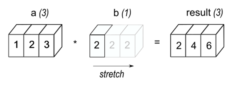
NumPy 的广播（Broadcasting） 是一种机制，用于处理不同形状（shape）的数组之间的算术运算，它可以自动扩展较小的数组，使其与较大数组的形状兼容，从而避免显式的形状调整（如复制数据），提高运算效率。

核心原则：形状兼容规则

两个数组要进行广播，需满足以下条件（从最后一个维度开始逐一比较）： 

1. 两个数组的对应维度长度相等；
2. 或其中一个数组的对应维度长度为 1；
3. 若维度数量不同，维度较少的数组会在前面自动补 1（“维度扩展”），再按上述规则比较。 

如果所有维度都满足条件，则可以广播；否则会报错（ValueError: operands could not be broadcast together）。

广播的步骤

1. 对齐维度：将两个数组的维度从右向左对齐（维度少的数组前面补 1）。
2. 扩展维度：将长度为 1 的维度扩展为与另一个数组对应维度相同的长度（仅逻辑上扩展，不实际复制数据）。
3. 执行运算：扩展后形状相同，按元素逐一运算。

示例说明

示例 1：标量与数组的广播

标量可视为 0 维数组，会被广播到与数组相同的形状：

import numpy as np
a = np.array([1, 2, 3])  # 形状 (3,)
b = 2                    # 标量，可视为形状 ()
c = a + b                # 广播后 b 视为 (3,)，结果 [3, 4, 5] 

示例 2：一维数组与二维数组的广播

a = np.array([[1, 2, 3],
              [4, 5, 6]])  # 形状 (2, 3)
b = np.array([10, 20, 30])  # 形状 (3,)

# 对齐维度：a 是 (2,3)，b 补维度后是 (1,3)
# 扩展 b 的第 0 维（长度 1→2），与 a 形状一致 (2,3)
c = a + b  # 结果：
# [[11, 22, 33],
#  [14, 25, 36]] 

示例 3：两个二维数组的广播

a = np.array([[1], [2], [3]])  # 形状 (3, 1)
b = np.array([[10, 20]])       # 形状 (1, 2)

# 对齐维度：a (3,1)，b (1,2)
# 扩展 a 的第 1 维（1→2），扩展 b 的第 0 维（1→3），最终均为 (3,2)
c = a + b  # 结果：
# [[11, 21],
#  [12, 22],
#  [13, 23]]

 

不兼容的情况

若维度既不相等也不为 1，则无法广播： 

a = np.array([[1, 2, 3]])  # 形状 (1, 3)
b = np.array([[1, 2]])     # 形状 (1, 2)
a + b  # 报错：最后一维 3 vs 2，不兼容

 

Advanced indexing and index tricks 高级索引和索引技巧

NumPy offers more indexing facilities than regular Python sequences. In addition to indexing by integers and slices, as we saw before, arrays can be indexed by arrays of integers and arrays of booleans. -- NumPy 提供了比常规 Python 序列更多的索引功能。除了之前提到的整数和切片索引之外，数组还可以通过整数数组和布尔数组进行索引。

>>> a = np.arange ( 12 ) ** 2
>>> a
array( [  0,   1,   4,   9,  16,  25,  36,  49,  64,  81, 100, 121 ] )

>>> i = np.array ( [ 1, 1, 3, 8, 5 ] )
>>> a [ i ]
array( [ 1,  1,  9, 64, 25 ] )

>>> j = np.array( [ [ 3, 4 ], [ 9, 7 ] ] )
>>> a [ j ]
array( [ [ 9, 16 ],
       [ 81, 49 ] ] )

 

上面这段这段代码展示了 NumPy 中的数组索引（高级索引） 功能，即通过另一个数组（索引数组）来选取原数组中的元素，具体解释如下：

1. 初始数组 a 的创建

a = np.arange(12) ** 2  

• np.arange(12) 生成 [0, 1, 2, ..., 11]（12 个元素的一维数组）。
• **2 对每个元素求平方，因此 a 的值为：

  array([  0,   1,   4,   9,  16,  25,  36,  49,  64,  81, 100, 121])  

2. 一维索引数组 i 选取元素

i = np.array([1, 1, 3, 8, 5])  # 索引数组（一维）
a[i]  # 用 i 中的元素作为索引，选取 a 中对应位置的元素  

• 索引数组 i 中的每个元素是 a 的索引：
  • i[0] = 1 → 对应 a[1] = 1
  • i[1] = 1 → 对应 a[1] = 1
  • i[2] = 3 → 对应 a[3] = 9
  • i[3] = 8 → 对应 a[8] = 64
  • i[4] = 5 → 对应 a[5] = 25
• 结果为：array([1, 1, 9, 64, 25])（形状与 i 相同，为一维数组）。

3. 二维索引数组 j 选取元素

j = np.array([[3, 4], [9, 7]])  # 索引数组（二维，2行2列）
a[j]  # 用 j 中的元素作为索引，选取 a 中对应位置的元素  

• 二维索引数组 j 的每个元素是 a 的索引，结果的形状与 j 一致（2 行 2 列）：
  • j[0,0] = 3 → a[3] = 9
  • j[0,1] = 4 → a[4] = 16
  • j[1,0] = 9 → a[9] = 81
  • j[1,1] = 7 → a[7] = 49
• 结果为：

  array([[ 9, 16],
         [81, 49]]) 

核心特点

• 索引数组的形状决定结果形状：无论索引数组是一维、二维还是更高维，选取结果的形状与索引数组完全一致。
• 允许重复索引：如 i 中两次出现 1，结果中会两次选取 a[1] 的值。
• 适用范围：这种方式属于 “高级索引”（与切片不同），适用于非连续、任意顺序的元素选取。 

通过数组索引，可灵活地从原数组中按指定顺序和形状选取元素，结果的结构与索引数组保持一致，是 NumPy 中高效提取数据的重要方式。

       

>>> a = np.arange(12).reshape(3,4)
>>> a
array( [ [  0,  1,  2,  3 ],
       [ 4,  5,  6,  7 ],
       [ 8,  9, 10, 11 ] ] )
>>> b = np.array ( [ [ 0, 1, 2 ], [ 2, 1, 0 ] ] )

>>> a [ b ]
array( [ [ [ 0,  1,  2,  3 ],
        [ 4,  5,  6,  7 ],
        [ 8,  9, 10, 11 ] ],

       [ [ 8,  9, 10, 11 ],
        [ 4,  5,  6,  7 ],
        [ 0,  1,  2,  3 ] ] ] )

When the indexed array “a” is multidimensional, a single array of indices refers to the first dimension of “a”. 当索引数组 a 为多维时，单个索引数组引用 a 的第一维。  

Tricks and tips 技巧和窍门

“Automatic” reshaping“自动”重塑
To change the dimensions of an array, you can omit one of the sizes which will then be deduced automatically 要更改数组的尺寸，您可以省略其中一个尺寸，系统将自动推断出该尺寸。

>>> a = np.arange(24)
>>> a
array( [ 0,  1,  2,  3,  4,  5,  6,  7,  8,  9, 10, 11, 12, 13, 14, 15, 16, 17, 18, 19, 20, 21, 22, 23 ] )
>>> b = a.reshape( ( 2, -1, 4 ) )
>>> b.shape
( 2, 3, 4 )
>>> b
array( [ [ [ 0,  1,  2,  3 ],
        [ 4,  5,  6,  7 ],
        [ 8,  9, 10, 11 ] ],

       [ [ 12, 13, 14, 15 ],
        [ 16, 17, 18, 19 ],
        [ 20, 21, 22, 23 ] ] ] )