TensorFlow从入门到理解(六):可视化梯度下降
运行代码:
import tensorflow as tf
import numpy as np
import matplotlib.pyplot as plt
from mpl_toolkits.mplot3d import Axes3D
LR = 0.1
REAL_PARAMS = [1.2, 2.5]
INIT_PARAMS = [[5, 4],
[5, 1],
[2, 4.5]][2]
x = np.linspace(-1, 1, 200, dtype=np.float32) # x data
y_fun = lambda a, b: np.sin(b*np.cos(a*x))
tf_y_fun = lambda a, b: tf.sin(b*tf.cos(a*x))
noise = np.random.randn(200)/10
y = y_fun(*REAL_PARAMS) + noise # target
# tensorflow graph
a, b = [tf.Variable(initial_value=p, dtype=tf.float32) for p in INIT_PARAMS]
pred = tf_y_fun(a, b)
mse = tf.reduce_mean(tf.square(y-pred))
train_op = tf.train.GradientDescentOptimizer(LR).minimize(mse)
a_list, b_list, cost_list = [], [], []
with tf.Session() as sess:
sess.run(tf.global_variables_initializer())
for t in range(400):
a_, b_, mse_ = sess.run([a, b, mse])
a_list.append(a_); b_list.append(b_); cost_list.append(mse_) # record parameter changes
result, _ = sess.run([pred, train_op]) # training
# visualization codes:
print('a=', a_, 'b=', b_)
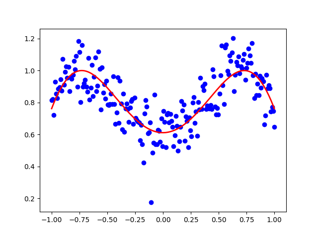
plt.figure(1)
plt.scatter(x, y, c='b') # plot data
plt.plot(x, result, 'r-', lw=2) # plot line fitting
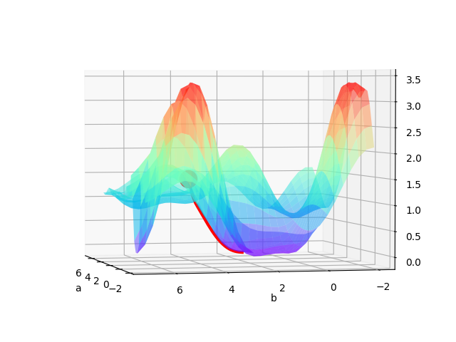
# 3D cost figure
fig = plt.figure(2); ax = Axes3D(fig)
a3D, b3D = np.meshgrid(np.linspace(-2, 7, 30), np.linspace(-2, 7, 30)) # parameter space
cost3D = np.array([np.mean(np.square(y_fun(a_, b_) - y)) for a_, b_ in zip(a3D.flatten(), b3D.flatten())]).reshape(a3D.shape)
ax.plot_surface(a3D, b3D, cost3D, rstride=1, cstride=1, cmap=plt.get_cmap('rainbow'), alpha=0.5)
ax.scatter(a_list[0], b_list[0], zs=cost_list[0], s=300, c='r') # initial parameter place
ax.set_xlabel('a'); ax.set_ylabel('b')
ax.plot(a_list, b_list, zs=cost_list, zdir='z', c='r', lw=3) # plot 3D gradient descent
plt.show()
运行结果:

 浙公网安备 33010602011771号