

人工智能 vgg
import tensorflow as tf
from tensorflow import keras
from tensorflow.keras import layers, regularizers
import numpy as np
import os
import cv2
import matplotlib.pyplot as plt
os.environ["CUDA_VISIBLE_DEVICES"] = "1"
resize = 224
path ="D:\anaconda\人工智能数据\第七章代码和数据\train"
def load_data():
imgs = os.listdir(path)
num = len(imgs)
train_data = np.empty((5000, resize, resize, 3), dtype="int32")
train_label = np.empty((5000, ), dtype="int32")
test_data = np.empty((5000, resize, resize, 3), dtype="int32")
test_label = np.empty((5000, ), dtype="int32")
for i in range(5000):
if i % 2:
train_data[i] = cv2.resize(cv2.imread(path+'/'+ 'dog.' + str(i) + '.jpg'), (resize, resize))
train_label[i] = 1
else:
train_data[i] = cv2.resize(cv2.imread(path+'/' + 'cat.' + str(i) + '.jpg'), (resize, resize))
train_label[i] = 0
for i in range(5000, 10000):
if i % 2:
test_data[i-5000] = cv2.resize(cv2.imread(path+'/' + 'dog.' + str(i) + '.jpg'), (resize, resize))
test_label[i-5000] = 1
else:
test_data[i-5000] = cv2.resize(cv2.imread(path+'/' + 'cat.' + str(i) + '.jpg'), (resize, resize))
test_label[i-5000] = 0
return train_data, train_label, test_data, test_label
def vgg16():
weight_decay = 0.0005
nb_epoch = 100
batch_size = 32
# layer1
model = keras.Sequential()
model.add(layers.Conv2D(64, (3, 3), padding='same',
input_shape=(224, 224, 3), kernel_regularizer=regularizers.l2(weight_decay)))
model.add(layers.Activation('relu'))
model.add(layers.BatchNormalization())
model.add(layers.Dropout(0.3))
# layer2
model.add(layers.Conv2D(64, (3, 3), padding='same', kernel_regularizer=regularizers.l2(weight_decay)))
model.add(layers.Activation('relu'))
model.add(layers.BatchNormalization())
model.add(layers.MaxPooling2D(pool_size=(2, 2)))
# layer3
model.add(layers.Conv2D(128, (3, 3), padding='same', kernel_regularizer=regularizers.l2(weight_decay)))
model.add(layers.Activation('relu'))
model.add(layers.BatchNormalization())
model.add(layers.Dropout(0.4))
# layer4
model.add(layers.Conv2D(128, (3, 3), padding='same', kernel_regularizer=regularizers.l2(weight_decay)))
model.add(layers.Activation('relu'))
model.add(layers.BatchNormalization())
model.add(layers.MaxPooling2D(pool_size=(2, 2)))
# layer5
model.add(layers.Conv2D(256, (3, 3), padding='same', kernel_regularizer=regularizers.l2(weight_decay)))
model.add(layers.Activation('relu'))
model.add(layers.BatchNormalization())
model.add(layers.Dropout(0.4))
# layer6
model.add(layers.Conv2D(256, (3, 3), padding='same', kernel_regularizer=regularizers.l2(weight_decay)))
model.add(layers.Activation('relu'))
model.add(layers.BatchNormalization())
model.add(layers.Dropout(0.4))
# layer7
model.add(layers.Conv2D(256, (3, 3), padding='same', kernel_regularizer=regularizers.l2(weight_decay)))
model.add(layers.Activation('relu'))
model.add(layers.BatchNormalization())
model.add(layers.MaxPooling2D(pool_size=(2, 2)))
# layer8
model.add(layers.Conv2D(512, (3, 3), padding='same', kernel_regularizer=regularizers.l2(weight_decay)))
model.add(layers.Activation('relu'))
model.add(layers.BatchNormalization())
model.add(layers.Dropout(0.4))
# layer9
model.add(layers.Conv2D(512, (3, 3), padding='same', kernel_regularizer=regularizers.l2(weight_decay)))
model.add(layers.Activation('relu'))
model.add(layers.BatchNormalization())
model.add(layers.Dropout(0.4))
# layer10
model.add(layers.Conv2D(512, (3, 3), padding='same', kernel_regularizer=regularizers.l2(weight_decay)))
model.add(layers.Activation('relu'))
model.add(layers.BatchNormalization())
model.add(layers.MaxPooling2D(pool_size=(2, 2)))
# layer11
model.add(layers.Conv2D(512, (3, 3), padding='same', kernel_regularizer=regularizers.l2(weight_decay)))
model.add(layers.Activation('relu'))
model.add(layers.BatchNormalization())
model.add(layers.Dropout(0.4))
# layer12
model.add(layers.Conv2D(512, (3, 3), padding='same', kernel_regularizer=regularizers.l2(weight_decay)))
model.add(layers.Activation('relu'))
model.add(layers.BatchNormalization())
model.add(layers.Dropout(0.4))
# layer13
model.add(layers.Conv2D(512, (3, 3), padding='same', kernel_regularizer=regularizers.l2(weight_decay)))
model.add(layers.Activation('relu'))
model.add(layers.BatchNormalization())
model.add(layers.MaxPooling2D(pool_size=(2, 2)))
model.add(layers.Dropout(0.5))
# layer14
model.add(layers.Flatten())
model.add(layers.Dense(512, kernel_regularizer=regularizers.l2(weight_decay)))
model.add(layers.Activation('relu'))
model.add(layers.BatchNormalization())
# layer15
model.add(layers.Dense(512, kernel_regularizer=regularizers.l2(weight_decay)))
model.add(layers.Activation('relu'))
model.add(layers.BatchNormalization())
# layer16
model.add(layers.Dropout(0.5))
model.add(layers.Dense(2))
model.add(layers.Activation('softmax'))
return model
#if __name__ == '__main__':
train_data, train_label, test_data, test_label = load_data()
train_data = train_data.astype('float32')
test_data = test_data.astype('float32')
train_label = keras.utils.to_categorical(train_label, 2)
test_label = keras.utils.to_categorical(test_label, 2)
#定义训练方法,超参数设置
model = vgg16()
sgd = tf.keras.optimizers.SGD(lr=0.01, decay=1e-6, momentum=0.9, nesterov=True) #设置优化器为SGD
model.compile(loss='categorical_crossentropy', optimizer=sgd, metrics=['accuracy'])
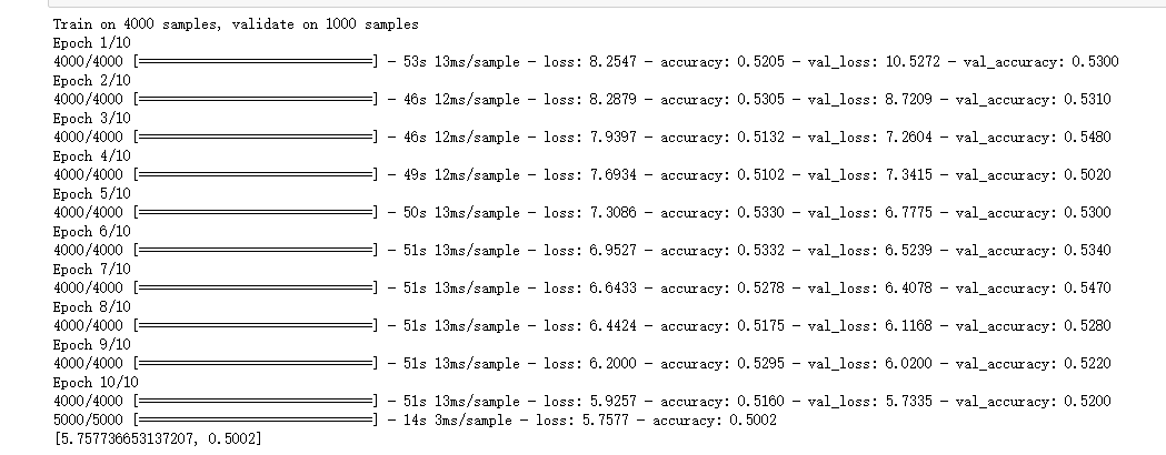
history = model.fit(train_data, train_label,
batch_size=20,
epochs=10,
validation_split=0.2, #把训练集中的五分之一作为验证集
shuffle=True)
scores = model.evaluate(test_data,test_label,verbose=1)
print(scores)
model.save('D:\anaconda\人工智能数据\第七章代码和数据\train')
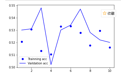
acc = history.history['accuracy'] # 获取训练集准确性数据
val_acc = history.history['val_accuracy'] # 获取验证集准确性数据
loss = history.history['loss'] # 获取训练集错误值数据
val_loss = history.history['val_loss'] # 获取验证集错误值数据
epochs = range(1, len(acc) + 1)
plt.plot(epochs, acc, 'bo', label='Trainning acc') # 以epochs为横坐标,以训练集准确性为纵坐标
plt.plot(epochs, val_acc, 'b', label='Vaildation acc') # 以epochs为横坐标,以验证集准确性为纵坐标
plt.legend() # 绘制图例,即标明图中的线段代表何种含义
plt.show()
结果截图:
网址代码:
# -*- coding: utf-8 -*-
"""
Neural Networks
===============
Neural networks can be constructed using the ``torch.nn`` package.
Now that you had a glimpse of ``autograd``, ``nn`` depends on
``autograd`` to define models and differentiate them.
An ``nn.Module`` contains layers, and a method ``forward(input)``\ that
returns the ``output``.
For example, look at this network that classifies digit images:
.. figure:: /_static/img/mnist.png
:alt: convnet
convnet
It is a simple feed-forward network. It takes the input, feeds it
through several layers one after the other, and then finally gives the
output.
A typical training procedure for a neural network is as follows:
- Define the neural network that has some learnable parameters (or
weights)
- Iterate over a dataset of inputs
- Process input through the network
- Compute the loss (how far is the output from being correct)
- Propagate gradients back into the network’s parameters
- Update the weights of the network, typically using a simple update rule:
``weight = weight - learning_rate * gradient``
Define the network
------------------
Let’s define this network:
"""
import torch
import torch.nn as nn
import torch.nn.functional as F
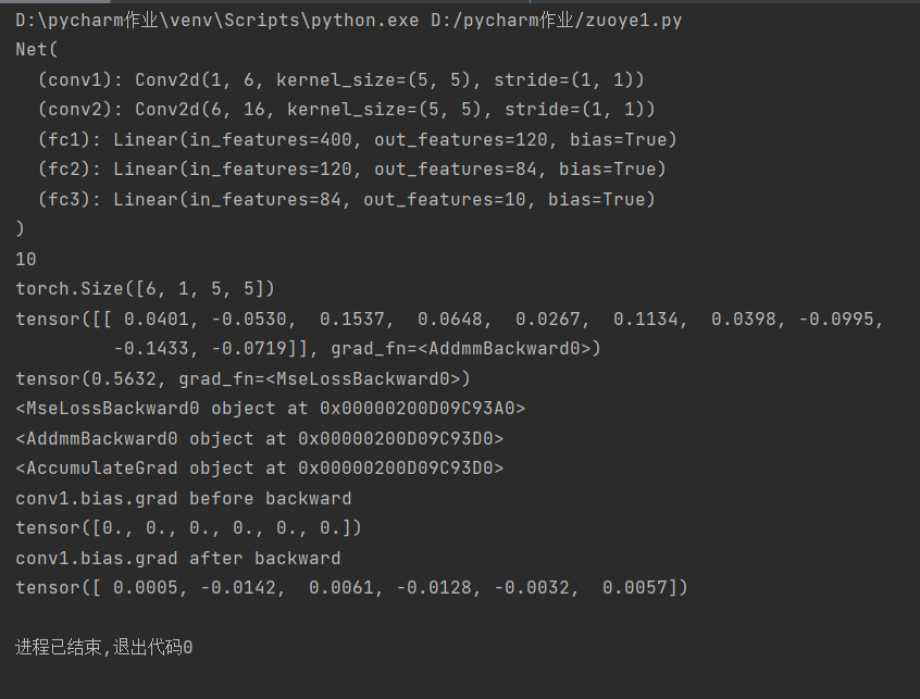
class Net(nn.Module):
def __init__(self):
super(Net, self).__init__()
# 1 input image channel, 6 output channels, 5x5 square convolution
# kernel
self.conv1 = nn.Conv2d(1, 6, 5)
self.conv2 = nn.Conv2d(6, 16, 5)
# an affine operation: y = Wx + b
self.fc1 = nn.Linear(16 * 5 * 5, 120)
self.fc2 = nn.Linear(120, 84)
self.fc3 = nn.Linear(84, 10)
def forward(self, x):
# Max pooling over a (2, 2) window
x = F.max_pool2d(F.relu(self.conv1(x)), (2, 2))
# If the size is a square you can only specify a single number
x = F.max_pool2d(F.relu(self.conv2(x)), 2)
x = x.view(-1, self.num_flat_features(x))
x = F.relu(self.fc1(x))
x = F.relu(self.fc2(x))
x = self.fc3(x)
return x
def num_flat_features(self, x):
size = x.size()[1:] # all dimensions except the batch dimension
num_features = 1
for s in size:
num_features *= s
return num_features
net = Net()
print(net)
########################################################################
# You just have to define the ``forward`` function, and the ``backward``
# function (where gradients are computed) is automatically defined for you
# using ``autograd``.
# You can use any of the Tensor operations in the ``forward`` function.
#
# The learnable parameters of a model are returned by ``net.parameters()``
params = list(net.parameters())
print(len(params))
print(params[0].size()) # conv1's .weight
########################################################################
# Let try a random 32x32 input
# Note: Expected input size to this net(LeNet) is 32x32. To use this net on
# MNIST dataset, please resize the images from the dataset to 32x32.
input = torch.randn(1, 1, 32, 32)
out = net(input)
print(out)
########################################################################
# Zero the gradient buffers of all parameters and backprops with random
# gradients:
net.zero_grad()
out.backward(torch.randn(1, 10))
########################################################################
# .. note::
#
# ``torch.nn`` only supports mini-batches. The entire ``torch.nn``
# package only supports inputs that are a mini-batch of samples, and not
# a single sample.
#
# For example, ``nn.Conv2d`` will take in a 4D Tensor of
# ``nSamples x nChannels x Height x Width``.
#
# If you have a single sample, just use ``input.unsqueeze(0)`` to add
# a fake batch dimension.
#
# Before proceeding further, let's recap all the classes you’ve seen so far.
#
# **Recap:**
# - ``torch.Tensor`` - A *multi-dimensional array* with support for autograd
# operations like ``backward()``. Also *holds the gradient* w.r.t. the
# tensor.
# - ``nn.Module`` - Neural network module. *Convenient way of
# encapsulating parameters*, with helpers for moving them to GPU,
# exporting, loading, etc.
# - ``nn.Parameter`` - A kind of Tensor, that is *automatically
# registered as a parameter when assigned as an attribute to a*
# ``Module``.
# - ``autograd.Function`` - Implements *forward and backward definitions
# of an autograd operation*. Every ``Tensor`` operation, creates at
# least a single ``Function`` node, that connects to functions that
# created a ``Tensor`` and *encodes its history*.
#
# **At this point, we covered:**
# - Defining a neural network
# - Processing inputs and calling backward
#
# **Still Left:**
# - Computing the loss
# - Updating the weights of the network
#
# Loss Function
# -------------
# A loss function takes the (output, target) pair of inputs, and computes a
# value that estimates how far away the output is from the target.
#
# There are several different
# `loss functions <https://pytorch.org/docs/nn.html#loss-functions>`_ under the
# nn package .
# A simple loss is: ``nn.MSELoss`` which computes the mean-squared error
# between the input and the target.
#
# For example:
output = net(input)
target = torch.randn(10) # a dummy target, for example
target = target.view(1, -1) # make it the same shape as output
criterion = nn.MSELoss()
loss = criterion(output, target)
print(loss)
########################################################################
# Now, if you follow ``loss`` in the backward direction, using its
# ``.grad_fn`` attribute, you will see a graph of computations that looks
# like this:
#
# ::
#
# input -> conv2d -> relu -> maxpool2d -> conv2d -> relu -> maxpool2d
# -> view -> linear -> relu -> linear -> relu -> linear
# -> MSELoss
# -> loss
#
# So, when we call ``loss.backward()``, the whole graph is differentiated
# w.r.t. the loss, and all Tensors in the graph that has ``requires_grad=True``
# will have their ``.grad`` Tensor accumulated with the gradient.
#
# For illustration, let us follow a few steps backward:
print(loss.grad_fn) # MSELoss
print(loss.grad_fn.next_functions[0][0]) # Linear
print(loss.grad_fn.next_functions[0][0].next_functions[0][0]) # ReLU
########################################################################
# Backprop
# --------
# To backpropagate the error all we have to do is to ``loss.backward()``.
# You need to clear the existing gradients though, else gradients will be
# accumulated to existing gradients.
#
#
# Now we shall call ``loss.backward()``, and have a look at conv1's bias
# gradients before and after the backward.
net.zero_grad() # zeroes the gradient buffers of all parameters
print('conv1.bias.grad before backward')
print(net.conv1.bias.grad)
loss.backward()
print('conv1.bias.grad after backward')
print(net.conv1.bias.grad)
########################################################################
# Now, we have seen how to use loss functions.
#
# **Read Later:**
#
# The neural network package contains various modules and loss functions
# that form the building blocks of deep neural networks. A full list with
# documentation is `here <https://pytorch.org/docs/nn>`_.
#
# **The only thing left to learn is:**
#
# - Updating the weights of the network
#
# Update the weights
# ------------------
# The simplest update rule used in practice is the Stochastic Gradient
# Descent (SGD):
#
# ``weight = weight - learning_rate * gradient``
#
# We can implement this using simple python code:
#
# .. code:: python
#
# learning_rate = 0.01
# for f in net.parameters():
# f.data.sub_(f.grad.data * learning_rate)
#
# However, as you use neural networks, you want to use various different
# update rules such as SGD, Nesterov-SGD, Adam, RMSProp, etc.
# To enable this, we built a small package: ``torch.optim`` that
# implements all these methods. Using it is very simple:
import torch.optim as optim
# create your optimizer
optimizer = optim.SGD(net.parameters(), lr=0.01)
# in your training loop:
optimizer.zero_grad() # zero the gradient buffers
output = net(input)
loss = criterion(output, target)
loss.backward()
optimizer.step() # Does the update
###############################################################
# .. Note::
#
# Observe how gradient buffers had to be manually set to zero using
# ``optimizer.zero_grad()``. This is because gradients are accumulated
# as explained in `Backprop`_ section.
结果截图:

 浙公网安备 33010602011771号