

TensorFlow学习报告
张量
张量是tensorflow中的基本数据结构,TensorFlow用张量这种数据结构来表示所有的数据.你可以把一个张量想象成一个n维的数组或列表.一个张量有一个静态类型和动态类型的维数.张量可以在图中的节点之间流通.其实张量更代表的就是一种多位数组。在tensorflow中,有很多操作张量的函数,有生成张量、创建随机张量、张量类型与形状变换和张量的切片与运算
改变类型
eg
tf.string_to_number(string_tensor, out_type=None, name=None)
tf.to_double(x, name='ToDouble')
tf.to_float(x, name='ToFloat')
tf.to_bfloat16(x, name='ToBFloat16')
tf.to_int32(x, name='ToInt32')
tf.to_int64(x, name='ToInt64')
tf.cast(x, dtype, name=None)
形状和变换
eg
tf.shape(input, name=None)
tf.size(input, name=None)
tf.rank(input, name=None)
tf.reshape(tensor, shape, name=None)
tf.squeeze(input, squeeze_dims=None, name=None)
tf.expand_dims(input, dim, name=None)
变量
变量的创建(定义)
Variable类
tf.Variable.init(initial_value, trainable=True, collections=None, validate_shape=True, name=None)
变量的初始化
变量的初始化必须在模型的其它操作运行之前先明确地完成。最简单的方法就是添加一个给所有变量初始化的操作,并在使用模型之前首先运行那个操作。最常见的初始化模式是使用便利函数 initialize_all_variables()将Op添加到初始化所有变量的图形中。
init = tf.global_variables_initializer()
开始会话
with tf.Session() as sess:
sess.run(init)
print(sess.run(c))
练习
1、局部连接:层间神经只有局部范围内的连接,在这个范围内采用全连接的方式,超过这个范围的神经元则没有连接;连接与连接之间独立参数,相比于去全连接减少了感受域外的连接,有效减少参数规模。
全连接:层间神经元完全连接,每个输出神经元可以获取到所有神经元的信息,有利于信息汇总,常置于网络末尾;连接与连接之间独立参数,大量的连接大大增加模型的参数规模。
2、 利用快速傅里叶变换把图片和卷积核变换到频域,频域把两者相乘,把结果利用傅里叶逆变换得到特征图。
3、池化操作作用:池化层同样基于局部相关性的思想,通过从局部相关的一组元素中进行采样或信息聚合,从而得到新的元素值。
激活函数作用:将A-NN模型中一个节点的输入信号转换成一个输出信号。该输出信号现在被用作堆叠中下一个层的输入。
4、局部归一化的作用:对局部神经元的活动创建了竞争环境,使得其中响应比较大的值变得相对更大,并抑制其他反馈较小的神经元,增强了模型的泛华能力。
5、 寻找损失函数的最低点,就像我们在山谷里行走,希望找到山谷里最低的地方。那么如何寻找损失函数的最低点呢?在这里,我们使用了微积分里导数,通过求出函数导数的值,从而找到函数下降的方向或者是最低点(极值点)。损失函数里一般有两种参数,一种是控制输入信号量的权重(Weight, 简称 ),另一种是调整函数与真实值距离的偏差(Bias,简称
)。我们所要做的工作,就是通过梯度下降方法,不断地调整权重
和偏差b,使得损失函数的值变得越来越小。而随机梯度下降算法只随机抽取一个样本进行梯度计算。
import tensorflow as tf
from tensorflow import keras
# Helper libraries
import numpy as np
import matplotlib.pyplot as plt
#导入数据集
print(tf.__version__)
fashion_mnist = keras.datasets.fashion_mnist
#浏览数据
(train_images, train_labels), (test_images, test_labels) = fashion_mnist.load_data()
fashion_mnist = keras.datasets.fashion_mnist
class_names = ['T-shirt/top', 'Trouser', 'Pullover', 'Dress', 'Coat',
'Sandal', 'Shirt', 'Sneaker', 'Bag', 'Ankle boot']
len(train_labels)
#预处理数据
len(test_labels)
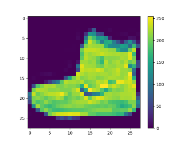
plt.figure()
plt.imshow(train_images[0])
plt.colorbar()
plt.grid(False)
plt.show()
train_images = train_images / 255.0
test_images = test_images / 255.0
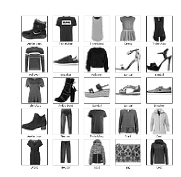
plt.figure(figsize=(10,10))
for i in range(25):
plt.subplot(5,5,i+1)
plt.xticks([])
plt.yticks([])
plt.grid(False)
plt.imshow(train_images[i], cmap=plt.cm.binary)
plt.xlabel(class_names[train_labels[i]])
plt.show()
#构建模型
model = keras.Sequential([
keras.layers.Flatten(input_shape=(28, 28)),
keras.layers.Dense(128, activation='relu'),
keras.layers.Dense(10)
])
#训练模型
model.compile(optimizer='adam',
loss=tf.keras.losses.SparseCategoricalCrossentropy(from_logits=True),
metrics=['accuracy'])
model.fit(train_images, train_labels, epochs=10)
#评估准确率
test_loss, test_acc = model.evaluate(test_images, test_labels, verbose=2)
print('\nTest accuracy:', test_acc)
probability_model = tf.keras.Sequential([model,
tf.keras.layers.Softmax()])
predictions = probability_model.predict(test_images)
np.argmax(predictions[0])
def plot_image(i, predictions_array, true_label, img):
predictions_array, true_label, img = predictions_array, true_label[i], img[i]
plt.grid(False)
plt.xticks([])
plt.yticks([])
plt.imshow(img, cmap=plt.cm.binary)
predicted_label = np.argmax(predictions_array)
if predicted_label == true_label:
color = 'blue'
else:
color = 'red'
plt.xlabel("{} {:2.0f}% ({})".format(class_names[predicted_label],
100*np.max(predictions_array),
class_names[true_label]),
color=color)
def plot_value_array(i, predictions_array, true_label):
predictions_array, true_label = predictions_array, true_label[i]
plt.grid(False)
plt.xticks(range(10))
plt.yticks([])
thisplot = plt.bar(range(10), predictions_array, color="#777777")
plt.ylim([0, 1])
predicted_label = np.argmax(predictions_array)
thisplot[predicted_label].set_color('red')
thisplot[true_label].set_color('blue')
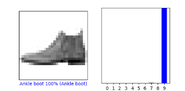
i = 0
plt.figure(figsize=(6, 3))
plt.subplot(1, 2, 1)
plot_image(i, predictions[i], test_labels, test_images)
plt.subplot(1, 2, 2)
plot_value_array(i, predictions[i], test_labels)
plt.show()
i = 12
plt.figure(figsize=(6, 3))
plt.subplot(1, 2, 1)
plot_image(i, predictions[i], test_labels, test_images)
plt.subplot(1, 2, 2)
plot_value_array(i, predictions[i], test_labels)
plt.show()
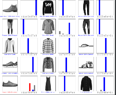
# Plot the first X test images, their predicted labels, and the true labels.
# Color correct predictions in blue and incorrect predictions in red.
num_rows = 5
num_cols = 3
num_images = num_rows * num_cols
plt.figure(figsize=(2 * 2 * num_cols, 2 * num_rows))
for i in range(num_images):
plt.subplot(num_rows, 2 * num_cols, 2 * i + 1)
plot_image(i, predictions[i], test_labels, test_images)
plt.subplot(num_rows, 2 * num_cols, 2 * i + 2)
plot_value_array(i, predictions[i], test_labels)
plt.tight_layout()
plt.show()
# Grab an image from the test dataset.
img = test_images[1]
print(img.shape)
# Add the image to a batch where it's the only member.
img = (np.expand_dims(img, 0))
print(img.shape)
predictions_single = probability_model.predict(img)
print(predictions_single)
plot_value_array(1, predictions_single[0], test_labels)
_ = plt.xticks(range(10), class_names, rotation=45)
np.argmax(predictions_single[0])

 浙公网安备 33010602011771号