信用评分卡（一）

目录

1. 导入数据
2. 缺失值和异常值处理
3. 特征可视化
4. 特征选择
5. 模型训练
6. 模型评估
7. 模型结果转评分
8. 计算用户总分

 

一、导入数据

#导入模块
import pandas as pd 
import numpy as np
from scipy import stats
import seaborn as sns
import matplotlib.pyplot as plt
%matplotlib inline
plt.rc("font",family="SimHei",size="12")  #解决中文无法显示的问题

#导入数据
train=pd.read_csv('F:\\python\\Give-me-some-credit-master\\data\\cs-training.csv')

 

数据信息简单查看 

#简单查看数据
train.info()

'''
train.info()
<class 'pandas.core.frame.DataFrame'>
RangeIndex: 150000 entries, 0 to 149999
Data columns (total 12 columns):
Unnamed: 0                              150000 non-null int64
SeriousDlqin2yrs                        150000 non-null int64
RevolvingUtilizationOfUnsecuredLines    150000 non-null float64
age                                     150000 non-null int64
NumberOfTime30-59DaysPastDueNotWorse    150000 non-null int64
DebtRatio                               150000 non-null float64
MonthlyIncome                           120269 non-null float64
NumberOfOpenCreditLinesAndLoans         150000 non-null int64
NumberOfTimes90DaysLate                 150000 non-null int64
NumberRealEstateLoansOrLines            150000 non-null int64
NumberOfTime60-89DaysPastDueNotWorse    150000 non-null int64
NumberOfDependents                      146076 non-null float64
dtypes: float64(4), int64(8)
memory usage: 13.7 MB

'''

 

头三行和末尾三行数据查看

#头三行和尾三行数据查看
train.head(3).append(train.tail(3))

 

shape查看

#shape
train.shape  #(150000, 11)

 

将各英文字段转为中文字段名方便理解

states={'Unnamed: 0':'id',
        'SeriousDlqin2yrs':'好坏客户',
        'RevolvingUtilizationOfUnsecuredLines':'可用额度比值',
        'age':'年龄',
        'NumberOfTime30-59DaysPastDueNotWorse':'逾期30-59天笔数',
        'DebtRatio':'负债率',
        'MonthlyIncome':'月收入',
        'NumberOfOpenCreditLinesAndLoans':'信贷数量',
        'NumberOfTimes90DaysLate':'逾期90天笔数',
        'NumberRealEstateLoansOrLines':'固定资产贷款量',
        'NumberOfTime60-89DaysPastDueNotWorse':'逾期60-89天笔数',
        'NumberOfDependents':'家属数量'}
train.rename(columns=states,inplace=True)

#设置索引
train=train.set_index('id',drop=True)

 

描述性统计

#描述性统计
train.describe()

 

 

二、缺失值和异常值处理

 

1.缺失值处理

  查看缺失值

#查看每列缺失情况
train.isnull().sum()
#查看缺失占比情况
train.isnull().sum()/len(train)
#缺失值可视化
missing=train.isnull().sum()
missing[missing>0].sort_values().plot.bar()  #将大于0的拿出来并排序

可知
月收入缺失值是：29731，缺失比例是：0.198207
家属数量缺失值：3924，缺失比例是：0.026160

先copy一份数据，保留原数据，然后对缺失值进行处理

#保留原数据
train_cp=train.copy()

#月收入使用平均值填补缺失值
train_cp.fillna({'月收入':train_cp['月收入'].mean()},inplace=True)
train_cp.isnull().sum()

#家属数量缺失的行去掉
train_cp=train_cp.dropna()
train_cp.shape   #(146076, 11)

 

2.异常值处理

查看异常值

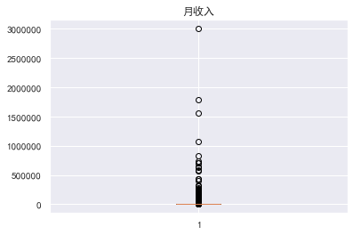
#查看异常值
#画箱型图
for col in train_cp.columns:
    plt.boxplot(train_cp[col])
    plt.title(col)
    plt.show()

可用额度比率大于1的数据是异常的

 

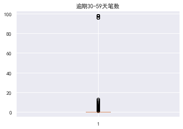
年龄为0的数据也是异常，其实小于18岁的都可以认定为异常，逾期30-59天笔数的有一个超级离群数据

 

 

 

 

 

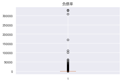
 异常值处理消除不合逻辑的数据和超级离群的数据，可用额度比值应该小于1，年龄为0的是异常值，逾期天数笔数大于80的是超级离群数据，将这些离群值过滤掉，筛选出剩余部分数据

train_cp=train_cp[train_cp['可用额度比值']<1]
train_cp=train_cp[train_cp['年龄']>0]
train_cp=train_cp[train_cp['逾期30-59天笔数']<80]
train_cp=train_cp[train_cp['逾期60-89天笔数']<80]
train_cp=train_cp[train_cp['逾期90天笔数']<80]
train_cp=train_cp[train_cp['固定资产贷款量']<50]
train_cp=train_cp[train_cp['负债率']<5000]
train_cp.shape  #(141180, 11)

 

 三、特征可视化

1.单变量可视化

好坏用户

#好坏用户
train_cp.info()
train_cp['好坏客户'].value_counts()
train_cp['好坏客户'].value_counts()/len(train_cp)
train_cp['好坏客户'].value_counts().plot.bar()

'''
0    132787
1      8393
Name: 好坏客户, dtype: int64
数据严重倾斜
0    0.940551
1    0.059449
Name: 好坏客户, dtype: float64

'''

 可知y值严重倾斜

 

可用额度比值和负债率

#可用额度比值和负债率
train_cp['可用额度比值'].plot.hist()
train_cp['负债率'].plot.hist()

 

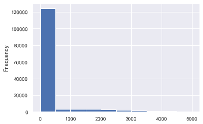
#负债率大于1的数据影响太大了
a=train_cp['负债率']
a[a<=1].plot.hist()

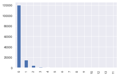
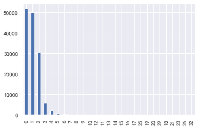
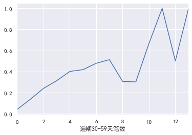
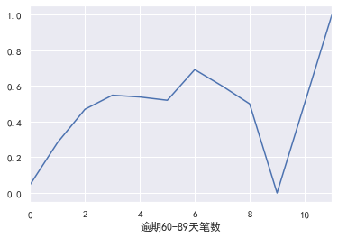
 逾期30-59天笔数,逾期90天笔数,逾期60-89天笔数

#逾期30-59天笔数,逾期90天笔数,逾期60-89天笔数 
for i,col in enumerate(['逾期30-59天笔数','逾期90天笔数','逾期60-89天笔数']):
    plt.subplot(1,3,i+1)
    train_cp[col].value_counts().plot.bar()
    plt.title(col)


train_cp['逾期30-59天笔数'].value_counts().plot.bar()
train_cp['逾期90天笔数'].value_counts().plot.bar()
train_cp['逾期60-89天笔数'].value_counts().plot.bar()

 

 年龄：基本符合正态分布

#年龄
train_cp['年龄'].plot.hist()

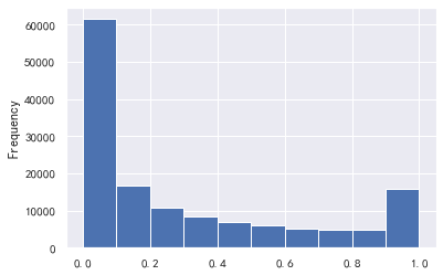
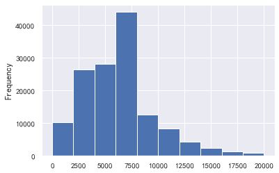
 月收入

#月收入
train_cp['月收入'].plot.hist()
sns.distplot(train_cp['月收入'])
#超级离群值影响太大了，我们取小于5w的数据画图
a=train_cp['月收入']
a[a<=50000].plot.hist()

#发现小于5万的也不多，那就取2w
a=train_cp['月收入']
a[a<=20000].plot.hist()

 

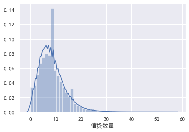
信贷数量

#信贷数量
train_cp['信贷数量'].value_counts().plot.bar()
sns.distplot(train_cp['信贷数量'])

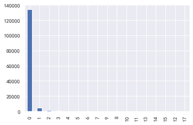
固定资产贷款量

#固定资产贷款量
train_cp['固定资产贷款量'].value_counts().plot.bar()
sns.distplot(train_cp['固定资产贷款量'])

家属数量

#家属数量
train_cp['家属数量'].value_counts().plot.bar()
sns.distplot(train_cp['家属数量'])

2.单变量与y值可视化

可用额度比值

#单变量与y值可视化
#可用额度比值、负债率、年龄、月收入，这些需要分箱
#可用额度比值
train_cp['可用额度比值_cut']=pd.cut(train_cp['可用额度比值'],5)
pd.crosstab(train_cp['可用额度比值_cut'],train_cp['好坏客户']).plot(kind="bar")
a=pd.crosstab(train_cp['可用额度比值_cut'],train_cp['好坏客户'])
a['坏用户占比']=a[1]/(a[0]+a[1])
a['坏用户占比'].plot()

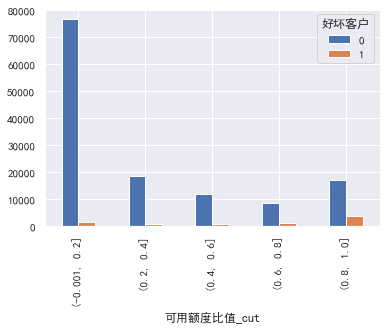
可见分箱最后的每个箱子的逾期率相差居然有6倍只差，说明该特征还是不错的

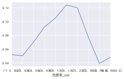
 负债率

#负债率
cut=[-1,0.2,0.4,0.6,0.8,1,1.5,2,5,10,5000]
train_cp['负债率_cut']=pd.cut(train_cp['负债率'],bins=cut)
pd.crosstab(train_cp['负债率_cut'],train_cp['好坏客户']).plot(kind="bar")
a=pd.crosstab(train_cp['负债率_cut'],train_cp['好坏客户'])
a['坏用户占比']=a[1]/(a[0]+a[1])
a['坏用户占比'].plot()

 年龄

#年龄
cut=[0,30,40,50,60,100]
train_cp['年龄_cut']=pd.cut(train_cp['年龄'],bins=cut)
pd.crosstab(train_cp['年龄_cut'],train_cp['好坏客户']).plot(kind="bar")
a=pd.crosstab(train_cp['年龄_cut'],train_cp['好坏客户'])
a['坏用户占比']=a[1]/(a[0]+a[1])
a['坏用户占比'].plot()

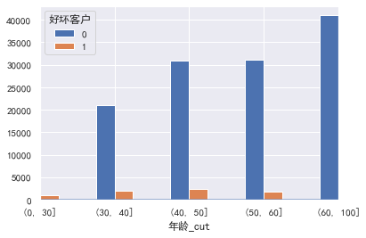
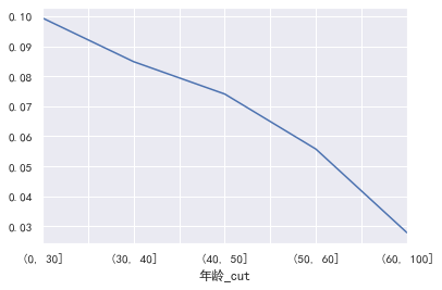
 为什么老年人这么多，不大现实吧，难道产品主要针对老年用户

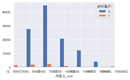
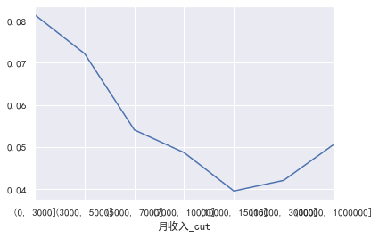
 月收入

#月收入
cut=[0,3000,5000,7000,10000,15000,30000,1000000]
train_cp['月收入_cut']=pd.cut(train_cp['月收入'],bins=cut)
pd.crosstab(train_cp['月收入_cut'],train_cp['好坏客户']).plot(kind="bar")
a=pd.crosstab(train_cp['月收入_cut'],train_cp['好坏客户'])
a['坏用户占比']=a[1]/(a[0]+a[1])
a['坏用户占比'].plot()

 逾期30-59天笔数,逾期90天笔数,逾期60-89天笔数 \信贷数量\固定资产贷款量\家属数量这些暂时不需要分箱：

 逾期30-59天笔数

#逾期30-59天笔数,逾期90天笔数,逾期60-89天笔数 \信贷数量\固定资产贷款量\家属数量
#逾期30-59天笔数
pd.crosstab(train_cp['逾期30-59天笔数'],train_cp['好坏客户']).plot(kind="bar")
a=pd.crosstab(train_cp['逾期30-59天笔数'],train_cp['好坏客户'])
a['坏用户占比']=a[1]/(a[0]+a[1])
a['坏用户占比'].plot()

 逾期90天笔数

#逾期90天笔数
pd.crosstab(train_cp['逾期90天笔数'],train_cp['好坏客户']).plot(kind="bar")
a=pd.crosstab(train_cp['逾期90天笔数'],train_cp['好坏客户'])
a['坏用户占比']=a[1]/(a[0]+a[1])
a['坏用户占比'].plot()

 

 逾期60-89天笔数

#逾期60-89天笔数
pd.crosstab(train_cp['逾期60-89天笔数'],train_cp['好坏客户']).plot(kind="bar")
a=pd.crosstab(train_cp['逾期60-89天笔数'],train_cp['好坏客户'])
a['坏用户占比']=a[1]/(a[0]+a[1])
a['坏用户占比'].plot()

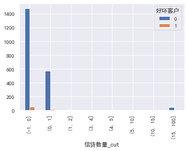
信贷数量

#信贷数量
cut=[-1,0,1,2,3,4,5,10,15,100]
train_cp['信贷数量_cut']=pd.cut(train_cp['月收入'],bins=cut)
pd.crosstab(train_cp['信贷数量_cut'],train_cp['好坏客户']).plot(kind="bar")
a=pd.crosstab(train_cp['信贷数量_cut'],train_cp['好坏客户'])
a['坏用户占比']=a[1]/(a[0]+a[1])
a['坏用户占比'].plot()

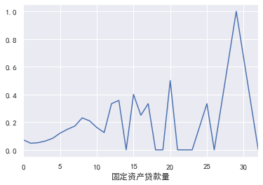
固定资产贷款量

#固定资产贷款量
pd.crosstab(train_cp['固定资产贷款量'],train_cp['好坏客户']).plot(kind="bar")
a=pd.crosstab(train_cp['固定资产贷款量'],train_cp['好坏客户'])
a['坏用户占比']=a[1]/(a[0]+a[1])
a['坏用户占比'].plot()

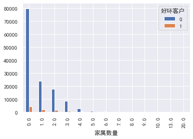
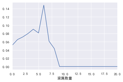
 家属数量

#家属数量
pd.crosstab(train_cp['家属数量'],train_cp['好坏客户']).plot(kind="bar")
a=pd.crosstab(train_cp['家属数量'],train_cp['好坏客户'])
a['坏用户占比']=a[1]/(a[0]+a[1])
a['坏用户占比'].plot()

 

3.变量之间的相关性：

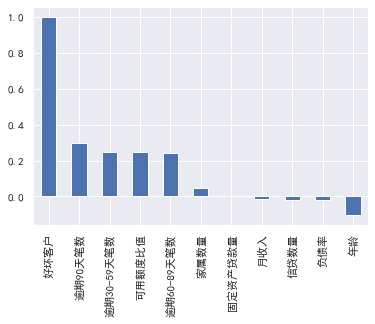
#变量之间的相关性
train_cp.corr()['好坏客户'].sort_values(ascending = False).plot(kind='bar')
plt.figure(figsize=(20,16))
corr=train_cp.corr()
sns.heatmap(corr, xticklabels=corr.columns, yticklabels=corr.columns, 
                 linewidths=0.2, cmap="YlGnBu",annot=True)

 

 

 

四、特征选择

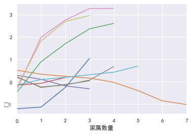
1.woe分箱

#woe分箱
cut1=pd.qcut(train_cp["可用额度比值"],4,labels=False)
cut2=pd.qcut(train_cp["年龄"],8,labels=False)
bins3=[-1,0,1,3,5,13]
cut3=pd.cut(train_cp["逾期30-59天笔数"],bins3,labels=False)
cut4=pd.qcut(train_cp["负债率"],3,labels=False)
cut5=pd.qcut(train_cp["月收入"],4,labels=False)
cut6=pd.qcut(train_cp["信贷数量"],4,labels=False)
bins7=[-1, 0, 1, 3,5, 20]
cut7=pd.cut(train_cp["逾期90天笔数"],bins7,labels=False)
bins8=[-1, 0,1,2, 3, 33]
cut8=pd.cut(train_cp["固定资产贷款量"],bins8,labels=False)
bins9=[-1, 0, 1, 3, 12]
cut9=pd.cut(train_cp["逾期60-89天笔数"],bins9,labels=False)
bins10=[-1, 0, 1, 2, 3, 5, 21]
cut10=pd.cut(train_cp["家属数量"],bins10,labels=False)

2.WOE值计算

当前这个组中坏客户和好客户的比值，和所有样本中这个比值的差异

#woe计算
rate=train_cp["好坏客户"].sum()/(train_cp["好坏客户"].count()-train_cp["好坏客户"].sum())  #rate=坏/(总-坏)
def get_woe_data(cut):
    grouped=train_cp["好坏客户"].groupby(cut,as_index = True).value_counts()
    woe=np.log(grouped.unstack().iloc[:,1]/grouped.unstack().iloc[:,0]/rate)
    return woe
cut1_woe=get_woe_data(cut1)
cut2_woe=get_woe_data(cut2)
cut3_woe=get_woe_data(cut3)
cut4_woe=get_woe_data(cut4)
cut5_woe=get_woe_data(cut5)
cut6_woe=get_woe_data(cut6)
cut7_woe=get_woe_data(cut7)
cut8_woe=get_woe_data(cut8)
cut9_woe=get_woe_data(cut9)
cut10_woe=get_woe_data(cut10)

可视化一下：

l=[cut1_woe,cut2_woe,cut3_woe,cut4_woe,cut5_woe,cut6_woe,cut7_woe,cut8_woe,cut9_woe,cut10_woe]
for i,col in enumerate(l):
    col.plot()
  

 3.iv值计算

iv值其实就等于woe*（当前分组中坏客户占所有坏客户的比例 - 当前分组中好客户占所有好客户的比例）

#iv值计算
def get_IV_data(cut,cut_woe):
    grouped=train_cp["好坏客户"].groupby(cut,as_index = True).value_counts()
    cut_IV=((grouped.unstack().iloc[:,1]/train_cp["好坏客户"].sum()-grouped.unstack().iloc[:,0]/(train_cp["好坏客户"].count()-train_cp["好坏客户"].sum()))*cut_woe).sum()    
    return cut_IV
#计算各分组的IV值
cut1_IV=get_IV_data(cut1,cut1_woe)
cut2_IV=get_IV_data(cut2,cut2_woe)
cut3_IV=get_IV_data(cut3,cut3_woe)
cut4_IV=get_IV_data(cut4,cut4_woe)
cut5_IV=get_IV_data(cut5,cut5_woe)
cut6_IV=get_IV_data(cut6,cut6_woe)
cut7_IV=get_IV_data(cut7,cut7_woe)
cut8_IV=get_IV_data(cut8,cut8_woe)
cut9_IV=get_IV_data(cut9,cut9_woe)
cut10_IV=get_IV_data(cut10,cut10_woe)
IV=pd.DataFrame([cut1_IV,cut2_IV,cut3_IV,cut4_IV,cut5_IV,cut6_IV,cut7_IV,cut8_IV,cut9_IV,cut10_IV],index=['可用额度比值','年龄','逾期30-59天笔数','负债率','月收入','信贷数量','逾期90天笔数','固定资产贷款量','逾期60-89天笔数','家属数量'],columns=['IV'])
iv=IV.plot.bar(color='b',alpha=0.3,rot=30,figsize=(10,5),fontsize=(10))
iv.set_title('特征变量与IV值分布图',fontsize=(15))
iv.set_xlabel('特征变量',fontsize=(15))
iv.set_ylabel('IV',fontsize=(15))

 

 

 一般选取IV大于0.02的特征变量进行后续训练，从以上可以看出所有变量均满足，所以选取全部的

4.woe转换

df_new=pd.DataFrame()   #新建df_new存放woe转换后的数据
def replace_data(cut,cut_woe):
    a=[]
    for i in cut.unique():
        a.append(i)
        a.sort()
    for m in range(len(a)):
        cut.replace(a[m],cut_woe.values[m],inplace=True)
    return cut
df_new["好坏客户"]=train_cp["好坏客户"]
df_new["可用额度比值"]=replace_data(cut1,cut1_woe)
df_new["年龄"]=replace_data(cut2,cut2_woe)
df_new["逾期30-59天笔数"]=replace_data(cut3,cut3_woe)
df_new["负债率"]=replace_data(cut4,cut4_woe)
df_new["月收入"]=replace_data(cut5,cut5_woe)
df_new["信贷数量"]=replace_data(cut6,cut6_woe)
df_new["逾期90天笔数"]=replace_data(cut7,cut7_woe)
df_new["固定资产贷款量"]=replace_data(cut8,cut8_woe)
df_new["逾期60-89天笔数"]=replace_data(cut9,cut9_woe)
df_new["家属数量"]=replace_data(cut10,cut10_woe)
df_new.head()

 

五、模型训练

信用评分卡主要使用的算法模型是逻辑回归。logistic模型客群变化的敏感度不如其他高复杂度模型，因此稳健更好，鲁棒性更强。另外，模型直观，系数含义好阐述、易理解，使用逻辑回归优点是可以得到一个变量之间的线性关系式和对应的特征权值，方便后面将其转成一一对应的分数形式

模型训练

#模型训练
from sklearn.linear_model import LogisticRegression
from sklearn.model_selection import train_test_split
x=df_new.iloc[:,1:]
y=df_new.iloc[:,:1]
x_train,x_test,y_train,y_test=train_test_split(x,y,test_size=0.6,random_state=0)
model=LogisticRegression()
clf=model.fit(x_train,y_train)
print('测试成绩：{}'.format(clf.score(x_test,y_test)))

测试成绩：0.9427326816829579，看似很高，其实是由于数据倾斜太严重导致，最终结果还要看auc

求特征权值系数coe，后面训练结果转分值时会用到：

coe=clf.coef_        #特征权值系数，后面转换为打分规则时会用到
coe

'''
array([[0.62805638, 0.46284749, 0.54319513, 1.14645109, 0.42744108,
        0.2503357 , 0.59564263, 0.81828033, 0.4433141 , 0.23788103]])
'''

 

六、模型评估

模型评估主要看AUC和K-S值

#模型评估
from sklearn.metrics import roc_curve, auc
fpr, tpr, threshold = roc_curve(y_test, y_pred)
roc_auc = auc(fpr, tpr)
plt.plot(fpr, tpr, color='darkorange',label='ROC curve (area = %0.2f)' % roc_auc)
plt.plot([0, 1], [0, 1], color='navy',  linestyle='--')
plt.xlim([0.0, 1.0])
plt.ylim([0.0, 1.0])
plt.xlabel('False Positive Rate')
plt.ylabel('True Positive Rate')
plt.title('ROC_curve')
plt.legend(loc="lower right")
plt.show()
 
roc_auc   #0.5756615527156178

 ks

#ks
fig, ax = plt.subplots()
ax.plot(1 - threshold, tpr, label='tpr') # ks曲线要按照预测概率降序排列，所以需要1-threshold镜像
ax.plot(1 - threshold, fpr, label='fpr')
ax.plot(1 - threshold, tpr-fpr,label='KS')
plt.xlabel('score')
plt.title('KS Curve')
plt.ylim([0.0, 1.0])
plt.figure(figsize=(20,20))
legend = ax.legend(loc='upper left')
plt.show()

max(tpr-fpr)  # 0.1513231054312355

 

 ROC0.58， K-S值0.15左右，建模效果一般

为什么分数这么高但是auc和ks很低，那是样本不均衡导致的

 

七、模型结果转评分

假设好坏比为20的时候分数为600分，每高20分好坏比翻一倍
现在我们求每个变量不同woe值对应的分数刻度可得：

#模型结果转评分
factor = 20 / np.log(2)
offset = 600 - 20 * np.log(20) / np.log(2)
def get_score(coe,woe,factor):
    scores=[]
    for w in woe:
        score=round(coe*w*factor,0)
        scores.append(score)
    return scores
x1 = get_score(coe[0][0], cut1_woe, factor)
x2 = get_score(coe[0][1], cut2_woe, factor)
x3 = get_score(coe[0][2], cut3_woe, factor)
x4 = get_score(coe[0][3], cut4_woe, factor)
x5 = get_score(coe[0][4], cut5_woe, factor)
x6 = get_score(coe[0][5], cut6_woe, factor)
x7 = get_score(coe[0][6], cut7_woe, factor)
x8 = get_score(coe[0][7], cut8_woe, factor)
x9 = get_score(coe[0][8], cut9_woe, factor)
x10 = get_score(coe[0][9], cut10_woe, factor)
print("可用额度比值对应的分数:{}".format(x1))
print("年龄对应的分数:{}".format(x2))
print("逾期30-59天笔数对应的分数:{}".format(x3))
print("负债率对应的分数:{}".format(x4))
print("月收入对应的分数:{}".format(x5))
print("信贷数量对应的分数:{}".format(x6))
print("逾期90天笔数对应的分数:{}".format(x7))
print("固定资产贷款量对应的分数:{}".format(x8))
print("逾期60-89天笔数对应的分数:{}".format(x9))
print("家属数量对应的分数:{}".format(x10))
 

 

可用额度比值对应的分数:[-22.0, -21.0, -5.0, 19.0]
年龄对应的分数:[7.0, 5.0, 3.0, 2.0, -0.0, -5.0, -11.0, -14.0]
逾期30-59天笔数对应的分数:[-7.0, 14.0, 27.0, 37.0, 41.0]
负债率对应的分数:[-5.0, -2.0, 6.0]
月收入对应的分数:[4.0, 1.0, -2.0, -4.0]
信贷数量对应的分数:[2.0, -2.0, -1.0, 0.0]
逾期90天笔数对应的分数:[-6.0, 34.0, 48.0, 56.0, 57.0]
固定资产贷款量对应的分数:[5.0, -6.0, -3.0, 2.0, 16.0]
逾期60-89天笔数对应的分数:[-3.0, 23.0, 35.0, 38.0]
家属数量对应的分数:[-1.0, 1.0, 1.0, 2.0, 3.0, 5.0]

可以看出分数越高，成为坏客户的可能性越大。像年龄越大坏客率越低，可用额度比值、逾期笔数这几个变量的分数跨度较大对最后的总分有更大的影响，这些都印证了前面探索分析的结果。

 

八、计算用户总得分

1.取自动分箱的边界分割点

cu1=pd.qcut(train_cp["可用额度比值"],4,labels=False,retbins=True)
bins1=cu1[1]
cu2=pd.qcut(train_cp["年龄"],8,labels=False,retbins=True)
bins2=cu2[1]

# bins3=[-1,0,1,3,5,13]
# cut3=pd.cut(train_cp["逾期30-59天笔数"],bins3,labels=False)
cu4=pd.qcut(train_cp["负债率"],3,labels=False,retbins=True)
bins4=cu4[1]
cu5=pd.qcut(train_cp["月收入"],4,labels=False,retbins=True)
bins5=cu5[1]
cu6=pd.qcut(train_cp["信贷数量"],4,labels=False,retbins=True)
bins6=cu6[1]

2.各变量对应的分数求和，算出每个用户的总分

#.各变量对应的分数求和，算出每个用户的总分
def compute_score(series,bins,score):
    list = []
    i = 0
    while i < len(series):
        value = series[i]
        j = len(bins) - 2
        m = len(bins) - 2
        while j >= 0:
            if value >= bins[j]:
                j = -1
            else:
                j -= 1
                m -= 1
        list.append(score[m])
        i += 1
    return list
path2=r'F:\\python\\Give-me-some-credit-master\\data\\cs-test.csv'

test1 = pd.read_csv(path2)

test1['x1'] = pd.Series(compute_score(test1['RevolvingUtilizationOfUnsecuredLines'], bins1, x1))
test1['x2'] = pd.Series(compute_score(test1['age'], bins2, x2))
test1['x3'] = pd.Series(compute_score(test1['NumberOfTime30-59DaysPastDueNotWorse'], bins3, x3))
test1['x4'] = pd.Series(compute_score(test1['DebtRatio'], bins4, x4))
test1['x5'] = pd.Series(compute_score(test1['MonthlyIncome'], bins5, x5))
test1['x6'] = pd.Series(compute_score(test1['NumberOfOpenCreditLinesAndLoans'], bins6, x6))
test1['x7'] = pd.Series(compute_score(test1['NumberOfTimes90DaysLate'], bins7, x7))
test1['x8'] = pd.Series(compute_score(test1['NumberRealEstateLoansOrLines'], bins8, x8))
test1['x9'] = pd.Series(compute_score(test1['NumberOfTime60-89DaysPastDueNotWorse'], bins9, x9))
test1['x10'] = pd.Series(compute_score(test1['NumberOfDependents'], bins10, x10))
test1['Score'] = test1['x1']+test1['x2']+test1['x3']+test1['x4']+test1['x5']+test1['x6']+test1['x7']+test1['x8']+test1['x9']+test1['x10']+600
test1.to_csv(r'F:\\python\\Give-me-some-credit-master\\data\\ScoreData.csv', index=False)

文章转载：https://www.cnblogs.com/daliner/p/10268350.html

 全部代码：

# -*- coding: utf-8 -*-
"""
Created on Tue Aug 11 14:09:20 2020

@author: Admin
"""

#导入模块
import pandas as pd 
import numpy as np
from scipy import stats
import seaborn as sns
import matplotlib.pyplot as plt
%matplotlib inline
plt.rc("font",family="SimHei",size="12")  #解决中文无法显示的问题

#导入数据
train=pd.read_csv('F:\\python\\Give-me-some-credit-master\\data\\cs-training.csv')

#简单查看数据
train.info()

#头三行和尾三行数据查看
b=train.head(3).append(train.tail(3))

#shape
train.shape  #(150000, 11)

#将各英文字段转为中文字段名方便理解
states={'Unnamed: 0':'id',
        'SeriousDlqin2yrs':'好坏客户',
        'RevolvingUtilizationOfUnsecuredLines':'可用额度比值',
        'age':'年龄',
        'NumberOfTime30-59DaysPastDueNotWorse':'逾期30-59天笔数',
        'DebtRatio':'负债率',
        'MonthlyIncome':'月收入',
        'NumberOfOpenCreditLinesAndLoans':'信贷数量',
        'NumberOfTimes90DaysLate':'逾期90天笔数',
        'NumberRealEstateLoansOrLines':'固定资产贷款量',
        'NumberOfTime60-89DaysPastDueNotWorse':'逾期60-89天笔数',
        'NumberOfDependents':'家属数量'}
train.rename(columns=states,inplace=True)

#设置索引
train=train.set_index('id',drop=True)

#描述性统计
train.describe()

#查看每列缺失情况
train.isnull().sum()
#查看缺失占比情况
train.isnull().sum()/len(train)
#缺失值可视化
missing=train.isnull().sum()
missing[missing>0].sort_values().plot.bar()  #将大于0的拿出来并排序

#保留原数据
train_cp=train.copy()

#月收入使用平均值填补缺失值
train_cp.fillna({'月收入':train_cp['月收入'].mean()},inplace=True)
train_cp.isnull().sum()

#家属数量缺失的行去掉
train_cp=train_cp.dropna()
train_cp.shape   #(146076, 11)

#查看异常值
#画箱型图
for col in train_cp.columns:
    plt.boxplot(train_cp[col])
    plt.title(col)
    plt.show()
    
#异常值处理
train_cp=train_cp[train_cp['可用额度比值']<1]
train_cp=train_cp[train_cp['年龄']>0]
train_cp=train_cp[train_cp['逾期30-59天笔数']<80]
train_cp=train_cp[train_cp['逾期60-89天笔数']<80]
train_cp=train_cp[train_cp['逾期90天笔数']<80]
train_cp=train_cp[train_cp['固定资产贷款量']<50]
train_cp=train_cp[train_cp['负债率']<5000]
train_cp.shape  #(141180, 11)

#单变量分析
#好坏用户
train_cp.info()
train_cp['好坏客户'].value_counts()
train_cp['好坏客户'].value_counts()/len(train_cp)
train_cp['好坏客户'].value_counts().plot.bar()

#可用额度比值和负债率
train_cp['可用额度比值'].plot.hist()
train_cp['负债率'].plot.hist()
#负债率大于1的数据影响太大了
a=train_cp['负债率']
a[a<=1].plot.hist()

#逾期30-59天笔数,逾期90天笔数,逾期60-89天笔数 
for i,col in enumerate(['逾期30-59天笔数','逾期90天笔数','逾期60-89天笔数']):
    plt.subplot(1,3,i+1)
    train_cp[col].value_counts().plot.bar()
    plt.title(col)


train_cp['逾期30-59天笔数'].value_counts().plot.bar()
train_cp['逾期90天笔数'].value_counts().plot.bar()
train_cp['逾期60-89天笔数'].value_counts().plot.bar()


#年龄
train_cp['年龄'].plot.hist()

#月收入
train_cp['月收入'].plot.hist()
sns.distplot(train_cp['月收入'])
#超级离群值影响太大了，我们取小于5w的数据画图
a=train_cp['月收入']
a[a<=50000].plot.hist()

#发现小于5万的也不多，那就取2w
a=train_cp['月收入']
a[a<=20000].plot.hist()

#信贷数量
train_cp['信贷数量'].value_counts().plot.bar()
sns.distplot(train_cp['信贷数量'])

#固定资产贷款量
train_cp['固定资产贷款量'].value_counts().plot.bar()
sns.distplot(train_cp['固定资产贷款量'])

#家属数量
train_cp['家属数量'].value_counts().plot.bar()
sns.distplot(train_cp['家属数量'])

#单变量与y值可视化
#可用额度比值、负债率、年龄、月收入，这些需要分箱
#可用额度比值
train_cp['可用额度比值_cut']=pd.cut(train_cp['可用额度比值'],5)
pd.crosstab(train_cp['可用额度比值_cut'],train_cp['好坏客户']).plot(kind="bar")
a=pd.crosstab(train_cp['可用额度比值_cut'],train_cp['好坏客户'])
a['坏用户占比']=a[1]/(a[0]+a[1])
a['坏用户占比'].plot()

#负债率
cut=[-1,0.2,0.4,0.6,0.8,1,1.5,2,5,10,5000]
train_cp['负债率_cut']=pd.cut(train_cp['负债率'],bins=cut)
pd.crosstab(train_cp['负债率_cut'],train_cp['好坏客户']).plot(kind="bar")
a=pd.crosstab(train_cp['负债率_cut'],train_cp['好坏客户'])
a['坏用户占比']=a[1]/(a[0]+a[1])
a['坏用户占比'].plot()

#年龄
cut=[0,30,40,50,60,100]
train_cp['年龄_cut']=pd.cut(train_cp['年龄'],bins=cut)
pd.crosstab(train_cp['年龄_cut'],train_cp['好坏客户']).plot(kind="bar")
a=pd.crosstab(train_cp['年龄_cut'],train_cp['好坏客户'])
a['坏用户占比']=a[1]/(a[0]+a[1])
a['坏用户占比'].plot()

#月收入
cut=[0,3000,5000,7000,10000,15000,30000,1000000]
train_cp['月收入_cut']=pd.cut(train_cp['月收入'],bins=cut)
pd.crosstab(train_cp['月收入_cut'],train_cp['好坏客户']).plot(kind="bar")
a=pd.crosstab(train_cp['月收入_cut'],train_cp['好坏客户'])
a['坏用户占比']=a[1]/(a[0]+a[1])
a['坏用户占比'].plot()

#逾期30-59天笔数,逾期90天笔数,逾期60-89天笔数 \信贷数量\固定资产贷款量\家属数量
#逾期30-59天笔数
pd.crosstab(train_cp['逾期30-59天笔数'],train_cp['好坏客户']).plot(kind="bar")
a=pd.crosstab(train_cp['逾期30-59天笔数'],train_cp['好坏客户'])
a['坏用户占比']=a[1]/(a[0]+a[1])
a['坏用户占比'].plot()

#逾期90天笔数
pd.crosstab(train_cp['逾期90天笔数'],train_cp['好坏客户']).plot(kind="bar")
a=pd.crosstab(train_cp['逾期90天笔数'],train_cp['好坏客户'])
a['坏用户占比']=a[1]/(a[0]+a[1])
a['坏用户占比'].plot()

#逾期60-89天笔数
pd.crosstab(train_cp['逾期60-89天笔数'],train_cp['好坏客户']).plot(kind="bar")
a=pd.crosstab(train_cp['逾期60-89天笔数'],train_cp['好坏客户'])
a['坏用户占比']=a[1]/(a[0]+a[1])
a['坏用户占比'].plot()

#信贷数量
cut=[-1,0,1,2,3,4,5,10,15,100]
train_cp['信贷数量_cut']=pd.cut(train_cp['月收入'],bins=cut)
pd.crosstab(train_cp['信贷数量_cut'],train_cp['好坏客户']).plot(kind="bar")
a=pd.crosstab(train_cp['信贷数量_cut'],train_cp['好坏客户'])
a['坏用户占比']=a[1]/(a[0]+a[1])
a['坏用户占比'].plot()

#固定资产贷款量
pd.crosstab(train_cp['固定资产贷款量'],train_cp['好坏客户']).plot(kind="bar")
a=pd.crosstab(train_cp['固定资产贷款量'],train_cp['好坏客户'])
a['坏用户占比']=a[1]/(a[0]+a[1])
a['坏用户占比'].plot()


#家属数量
pd.crosstab(train_cp['家属数量'],train_cp['好坏客户']).plot(kind="bar")
a=pd.crosstab(train_cp['家属数量'],train_cp['好坏客户'])
a['坏用户占比']=a[1]/(a[0]+a[1])
a['坏用户占比'].plot()


#变量之间的相关性
train_cp.corr()['好坏客户'].sort_values(ascending = False).plot(kind='bar')
plt.figure(figsize=(20,16))
corr=train_cp.corr()
sns.heatmap(corr, xticklabels=corr.columns, yticklabels=corr.columns, 
                 linewidths=0.2, cmap="YlGnBu",annot=True)

#woe分箱
cut1=pd.qcut(train_cp["可用额度比值"],4,labels=False)
cut2=pd.qcut(train_cp["年龄"],8,labels=False)
bins3=[-1,0,1,3,5,13]
cut3=pd.cut(train_cp["逾期30-59天笔数"],bins3,labels=False)
cut4=pd.qcut(train_cp["负债率"],3,labels=False)
cut5=pd.qcut(train_cp["月收入"],4,labels=False)
cut6=pd.qcut(train_cp["信贷数量"],4,labels=False)
bins7=[-1, 0, 1, 3,5, 20]
cut7=pd.cut(train_cp["逾期90天笔数"],bins7,labels=False)
bins8=[-1, 0,1,2, 3, 33]
cut8=pd.cut(train_cp["固定资产贷款量"],bins8,labels=False)
bins9=[-1, 0, 1, 3, 12]
cut9=pd.cut(train_cp["逾期60-89天笔数"],bins9,labels=False)
bins10=[-1, 0, 1, 2, 3, 5, 21]
cut10=pd.cut(train_cp["家属数量"],bins10,labels=False)

#woe计算
rate=train_cp["好坏客户"].sum()/(train_cp["好坏客户"].count()-train_cp["好坏客户"].sum())  #rate=坏/(总-坏)
def get_woe_data(cut):
    grouped=train_cp["好坏客户"].groupby(cut,as_index = True).value_counts()
    woe=np.log(grouped.unstack().iloc[:,1]/grouped.unstack().iloc[:,0]/rate)
    return woe
cut1_woe=get_woe_data(cut1)
cut2_woe=get_woe_data(cut2)
cut3_woe=get_woe_data(cut3)
cut4_woe=get_woe_data(cut4)
cut5_woe=get_woe_data(cut5)
cut6_woe=get_woe_data(cut6)
cut7_woe=get_woe_data(cut7)
cut8_woe=get_woe_data(cut8)
cut9_woe=get_woe_data(cut9)
cut10_woe=get_woe_data(cut10)

l=[cut1_woe,cut2_woe,cut3_woe,cut4_woe,cut5_woe,cut6_woe,cut7_woe,cut8_woe,cut9_woe,cut10_woe]
for i,col in enumerate(l):
    col.plot()
  

#iv值计算
def get_IV_data(cut,cut_woe):
    grouped=train_cp["好坏客户"].groupby(cut,as_index = True).value_counts()
    cut_IV=((grouped.unstack().iloc[:,1]/train_cp["好坏客户"].sum()-grouped.unstack().iloc[:,0]/(train_cp["好坏客户"].count()-train_cp["好坏客户"].sum()))*cut_woe).sum()    
    return cut_IV
#计算各分组的IV值
cut1_IV=get_IV_data(cut1,cut1_woe)
cut2_IV=get_IV_data(cut2,cut2_woe)
cut3_IV=get_IV_data(cut3,cut3_woe)
cut4_IV=get_IV_data(cut4,cut4_woe)
cut5_IV=get_IV_data(cut5,cut5_woe)
cut6_IV=get_IV_data(cut6,cut6_woe)
cut7_IV=get_IV_data(cut7,cut7_woe)
cut8_IV=get_IV_data(cut8,cut8_woe)
cut9_IV=get_IV_data(cut9,cut9_woe)
cut10_IV=get_IV_data(cut10,cut10_woe)
IV=pd.DataFrame([cut1_IV,cut2_IV,cut3_IV,cut4_IV,cut5_IV,cut6_IV,cut7_IV,cut8_IV,cut9_IV,cut10_IV],index=['可用额度比值','年龄','逾期30-59天笔数','负债率','月收入','信贷数量','逾期90天笔数','固定资产贷款量','逾期60-89天笔数','家属数量'],columns=['IV'])
iv=IV.plot.bar(color='b',alpha=0.3,rot=30,figsize=(10,5),fontsize=(10))
iv.set_title('特征变量与IV值分布图',fontsize=(15))
iv.set_xlabel('特征变量',fontsize=(15))
iv.set_ylabel('IV',fontsize=(15))

#woe转换
df_new=pd.DataFrame()   #新建df_new存放woe转换后的数据
def replace_data(cut,cut_woe):
    a=[]
    for i in cut.unique():
        a.append(i)
        a.sort()
    for m in range(len(a)):
        cut.replace(a[m],cut_woe.values[m],inplace=True)
    return cut
df_new["好坏客户"]=train_cp["好坏客户"]
df_new["可用额度比值"]=replace_data(cut1,cut1_woe)
df_new["年龄"]=replace_data(cut2,cut2_woe)
df_new["逾期30-59天笔数"]=replace_data(cut3,cut3_woe)
df_new["负债率"]=replace_data(cut4,cut4_woe)
df_new["月收入"]=replace_data(cut5,cut5_woe)
df_new["信贷数量"]=replace_data(cut6,cut6_woe)
df_new["逾期90天笔数"]=replace_data(cut7,cut7_woe)
df_new["固定资产贷款量"]=replace_data(cut8,cut8_woe)
df_new["逾期60-89天笔数"]=replace_data(cut9,cut9_woe)
df_new["家属数量"]=replace_data(cut10,cut10_woe)
df_new.head()

#模型训练
from sklearn.linear_model import LogisticRegression
from sklearn.model_selection import train_test_split
x=df_new.iloc[:,1:]
y=df_new.iloc[:,:1]
x_train,x_test,y_train,y_test=train_test_split(x,y,test_size=0.6,random_state=0)
model=LogisticRegression()
clf=model.fit(x_train,y_train)
print('测试成绩：{}'.format(clf.score(x_test,y_test)))

#系数
coe=clf.coef_        #特征权值系数，后面转换为打分规则时会用到
coe

#测试集的分数
y_pred=clf.predict(x_test)

#模型评估
from sklearn.metrics import roc_curve, auc
fpr, tpr, threshold = roc_curve(y_test, y_pred)
roc_auc = auc(fpr, tpr)
plt.plot(fpr, tpr, color='darkorange',label='ROC curve (area = %0.2f)' % roc_auc)
plt.plot([0, 1], [0, 1], color='navy',  linestyle='--')
plt.xlim([0.0, 1.0])
plt.ylim([0.0, 1.0])
plt.xlabel('False Positive Rate')
plt.ylabel('True Positive Rate')
plt.title('ROC_curve')
plt.legend(loc="lower right")
plt.show()
 
roc_auc   #0.5756615527156178

#ks
fig, ax = plt.subplots()
ax.plot(1 - threshold, tpr, label='tpr') # ks曲线要按照预测概率降序排列，所以需要1-threshold镜像
ax.plot(1 - threshold, fpr, label='fpr')
ax.plot(1 - threshold, tpr-fpr,label='KS')
plt.xlabel('score')
plt.title('KS Curve')
plt.ylim([0.0, 1.0])
plt.figure(figsize=(20,20))
legend = ax.legend(loc='upper left')
plt.show()

max(tpr-fpr)  # 0.1513231054312355


#模型结果转评分
factor = 20 / np.log(2)
offset = 600 - 20 * np.log(20) / np.log(2)
def get_score(coe,woe,factor):
    scores=[]
    for w in woe:
        score=round(coe*w*factor,0)
        scores.append(score)
    return scores
x1 = get_score(coe[0][0], cut1_woe, factor)
x2 = get_score(coe[0][1], cut2_woe, factor)
x3 = get_score(coe[0][2], cut3_woe, factor)
x4 = get_score(coe[0][3], cut4_woe, factor)
x5 = get_score(coe[0][4], cut5_woe, factor)
x6 = get_score(coe[0][5], cut6_woe, factor)
x7 = get_score(coe[0][6], cut7_woe, factor)
x8 = get_score(coe[0][7], cut8_woe, factor)
x9 = get_score(coe[0][8], cut9_woe, factor)
x10 = get_score(coe[0][9], cut10_woe, factor)
print("可用额度比值对应的分数:{}".format(x1))
print("年龄对应的分数:{}".format(x2))
print("逾期30-59天笔数对应的分数:{}".format(x3))
print("负债率对应的分数:{}".format(x4))
print("月收入对应的分数:{}".format(x5))
print("信贷数量对应的分数:{}".format(x6))
print("逾期90天笔数对应的分数:{}".format(x7))
print("固定资产贷款量对应的分数:{}".format(x8))
print("逾期60-89天笔数对应的分数:{}".format(x9))
print("家属数量对应的分数:{}".format(x10))
 
#1.取自动分箱的边界分割点
cu1=pd.qcut(train_cp["可用额度比值"],4,labels=False,retbins=True)
bins1=cu1[1]
cu2=pd.qcut(train_cp["年龄"],8,labels=False,retbins=True)
bins2=cu2[1]

# bins3=[-1,0,1,3,5,13]
# cut3=pd.cut(train_cp["逾期30-59天笔数"],bins3,labels=False)
cu4=pd.qcut(train_cp["负债率"],3,labels=False,retbins=True)
bins4=cu4[1]
cu5=pd.qcut(train_cp["月收入"],4,labels=False,retbins=True)
bins5=cu5[1]
cu6=pd.qcut(train_cp["信贷数量"],4,labels=False,retbins=True)
bins6=cu6[1]


#.各变量对应的分数求和，算出每个用户的总分
def compute_score(series,bins,score):
    list = []
    i = 0
    while i < len(series):
        value = series[i]
        j = len(bins) - 2
        m = len(bins) - 2
        while j >= 0:
            if value >= bins[j]:
                j = -1
            else:
                j -= 1
                m -= 1
        list.append(score[m])
        i += 1
    return list
path2=r'F:\\python\\Give-me-some-credit-master\\data\\cs-test.csv'

test1 = pd.read_csv(path2)

test1['x1'] = pd.Series(compute_score(test1['RevolvingUtilizationOfUnsecuredLines'], bins1, x1))
test1['x2'] = pd.Series(compute_score(test1['age'], bins2, x2))
test1['x3'] = pd.Series(compute_score(test1['NumberOfTime30-59DaysPastDueNotWorse'], bins3, x3))
test1['x4'] = pd.Series(compute_score(test1['DebtRatio'], bins4, x4))
test1['x5'] = pd.Series(compute_score(test1['MonthlyIncome'], bins5, x5))
test1['x6'] = pd.Series(compute_score(test1['NumberOfOpenCreditLinesAndLoans'], bins6, x6))
test1['x7'] = pd.Series(compute_score(test1['NumberOfTimes90DaysLate'], bins7, x7))
test1['x8'] = pd.Series(compute_score(test1['NumberRealEstateLoansOrLines'], bins8, x8))
test1['x9'] = pd.Series(compute_score(test1['NumberOfTime60-89DaysPastDueNotWorse'], bins9, x9))
test1['x10'] = pd.Series(compute_score(test1['NumberOfDependents'], bins10, x10))
test1['Score'] = test1['x1']+test1['x2']+test1['x3']+test1['x4']+test1['x5']+test1['x6']+test1['x7']+test1['x8']+test1['x9']+test1['x10']+600
test1.to_csv(r'F:\\python\\Give-me-some-credit-master\\data\\ScoreData.csv', index=False)