
pandas 的groupby()
2022.10.08增加了25 个例子学会Pandas Groupby 操作! (qq.com)
groupby()
DataFrame.groupby(by=None, axis=0, level=None, as_index=True, sort=True, group_keys=True, squeeze=<object object>, observed=False, dropna=True)[source]
参数:
- by:mapping, function, label, or list of labels,用于确定groupby的组。如果by是函数,则在对象索引的每个值上调用它。如果通过了dict或Series,则将使用Series或dict VALUES来确定组,如果传递ndarray,则按原样使用这些值来确定组,和pd.cut()一起使用
- axis:{0 or ‘index’, 1 or ‘columns’}, default 0,沿行(0)或列(1)拆分
- level:int, level name, or sequence of such, default None,如果轴是MultiIndex(分层),则按一个或多个特定级别分组
- as_index:bool, default True,as_index决定了分组使用的属性是否成为新的表格的索引,as_index=False没有索引了
- sort:bool, default True,排序组键。关闭此功能可获得更好的性能
- group_keys:bool, default True,调用apply时,将组键添加到索引以识别片段
- squeeze:bool, default False,如果可能,请减小返回类型的维数,否则返回一致的类型,从1.1.0版开始不推荐使用
- observed:bool, default False,
- dropna:bool, default True,如果为True,并且如果组键包含NA值,则将删除NA值以及行/列。如果为False,则NA值也将被视为组中的键
返回:
DataFrameGroupBy对象
含义:as_index决定了分组使用的属性是否成为新的表格的索引,默认是as_index=True,我的代码中常用:as_index=False.
- 使用作为索引只是会影响查询速度,而一般没有这样的需求。
- as_index=True是常用的表格形式,而as_index=False除了表格有变化,显示也会不同,as_index=False没有索引了。
groupby函数可以将一个df (或者是 df[col] )根据某一列或者某几列分组又或者是函数 又或者是 (和df或者 df[col] 长度一样的 pd.series)分组,经过groupby后会生成一个groupby对象,该对象本身不会返回任何内容,只有当相应的方法被调用时才会起作用
- 根据某一列分组
- 根据某几列分组,和根据某列分组用法基本一致
- 查看组容量和组数(size)
- 组的遍历,得到的组内数据分别是一个个df
- head()和first()
- [col].数学统计变量,即是计算每个分组该列的数学统计值
- 聚合函数(mean/sum/size/count/std/var/sem/describe/first/last/nth/min/max)和agg
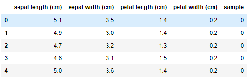
我们使用iris数据做例子
from sklearn.datasets import load_iris
import pandas as pd
import numpy as np
iris=load_iris()
df=pd.DataFrame(iris.data,columns=iris.feature_names)
df['sample']=iris.target
1.根据某一列分组
#根据sample分组
group_sample=df.groupby('sample')

#get_group()是查看某一分组,比如说上面的sample有三种类别,我们可以使用get_group()查看某一类别
group_sample.get_group(0).head()
2.根据某几列分组,和根据某列分组用法基本一致
#列名需要以list形式传入
group_n=df.groupby(['petal width (cm)', 'sample'])

group_n.get_group((0.1,0))
3.查看组容量和组数(size)
#调用get_group时可以先查看一个有几种分组,组内的容量是怎么样的
group_n.size()
petal width (cm)  sample
0.1               0          5
0.2               0         29
0.3               0          7
0.4               0          7
0.5               0          1
0.6               0          1
1.0               1          7
1.1               1          3
1.2               1          5
1.3               1         13
1.4               1          7
                  2          1
1.5               1         10
                  2          2
1.6               1          3
                  2          1
1.7               1          1
                  2          1
1.8               1          1
                  2         11
1.9               2          5
2.0               2          6
2.1               2          6
2.2               2          3
2.3               2          8
2.4               2          3
2.5               2          3
dtype: int64
4.组的遍历,得到的组内数据分别是一个个df
#name,group 分别是组名和组内数据
for name,group in group_n:
    print(name)
    print(group.head())
5.head()和first()
#head()返回的是每个组的前某几行,而不是数据集的前几行
group_n.head(2)

#first()返回的每个分组的第一行信息,组成了一个df
group_n.first()
6.[col].数学统计变量,即是计算每个分组该列的数学统计值
#计算每个分组的某列的平均值
group_n['sepal length (cm)'].mean()

#返回的布尔型的值
group_n['sepal length (cm)'].mean()>5
petal width (cm)  sample
0.1               0         4.820000
0.2               0         4.972414
0.3               0         4.971429
0.4               0         5.300000
0.5               0         5.100000
0.6               0         5.000000
1.0               1         5.414286
1.1               1         5.400000
1.2               1         5.780000
1.3               1         5.884615
1.4               1         6.357143
                  2         6.100000
1.5               1         6.190000
                  2         6.150000
1.6               1         6.100000
                  2         7.200000
1.7               1         6.700000
                  2         4.900000
1.8               1         5.900000
                  2         6.445455
1.9               2         6.340000
2.0               2         6.650000
2.1               2         6.916667
2.2               2         6.866667
2.3               2         6.912500
2.4               2         6.266667
2.5               2         6.733333
Name: sepal length (cm), dtype: float64
petal width (cm)  sample
0.1               0         False
0.2               0         False
0.3               0         False
0.4               0          True
0.5               0          True
0.6               0         False
1.0               1          True
1.1               1          True
1.2               1          True
1.3               1          True
1.4               1          True
                  2          True
1.5               1          True
                  2          True
1.6               1          True
                  2          True
1.7               1          True
                  2         False
1.8               1          True
                  2          True
1.9               2          True
2.0               2          True
2.1               2          True
2.2               2          True
2.3               2          True
2.4               2          True
2.5               2          True
Name: sepal length (cm), dtype: bool
7.聚合函数(mean/sum/size/count/std/var/sem/describe/first/last/nth/min/max),用法上面例子有,就不赘述了
下面主要说一下agg()同时使用多个聚合函数
#计算每组每个特征的平均值
group_n.mean()

#同时使用多个聚合函数
group_n.agg(('sum','mean'))
group_n.agg(['sum','mean'])

#和上面一样,只不过是重新命名了
group_n.agg([('rename_sum','sum'),('rename_mean','mean')])

#指定某一列使用某些函数,以字典形式传入
group_n.agg({'sepal length (cm)':['mean','max'],'sepal width (cm)':'var'})

#使用匿名函数或者自定义函数
group_n.agg(lambda x:x.max()-x.min())
下面补充一下df[col]根据series分组的例子:结合了value_counts,unstack()
#woe计算
cut1=pd.qcut(train_cp["可用额度比值"],4,labels=False)
rate=train_cp["好坏客户"].sum()/(train_cp["好坏客户"].count()-train_cp["好坏客户"].sum())  #rate=坏/(总-坏)
def get_woe_data(cut):
    grouped=train_cp["好坏客户"].groupby(cut,as_index = True).value_counts()
    woe=np.log(grouped.unstack().iloc[:,1]/grouped.unstack().iloc[:,0]/rate)
    return woe
cut1_woe=get_woe_data(cut1)
=========================================================
2021.2.26补充一下groupby.transform 的用法
In [90]: people
Out[90]:
               a         b         c         d         e
Joe     0.498185  0.460470 -0.892633 -1.561500  0.279949
Steve  -0.885170 -1.490421 -0.787302  1.559050  1.183115
Wes    -0.237464       NaN       NaN -0.043788 -1.091813
Jim    -1.547607 -0.121682 -0.355623 -1.703322 -0.733741
Travis  0.638562  0.486515 -0.233517  0.023372  0.366325

In [94]: key = list('ototo')

# 按键值key,计算均值

In [95]: people.groupby(key).mean()
Out[95]:
          a         b         c         d         e
o  0.299761  0.473492 -0.563075 -0.527305 -0.148513
t -1.216388 -0.806052 -0.571462 -0.072136  0.224687

# 把原数据转换为以上均值

In [96]: people.groupby(key).transform(np.mean)
Out[96]:
               a         b         c         d         e
Joe     0.299761  0.473492 -0.563075 -0.527305 -0.148513
Steve  -1.216388 -0.806052 -0.571462 -0.072136  0.224687
Wes     0.299761  0.473492 -0.563075 -0.527305 -0.148513
Jim    -1.216388 -0.806052 -0.571462 -0.072136  0.224687
Travis  0.299761  0.473492 -0.563075 -0.527305 -0.148513
总结一下就是可以使用groupby.transform将我们的原始数据替换成我们想要的均值中值等等

 浙公网安备 33010602011771号