NumPy 秘籍中文第二版：6~10

原文：NumPy Cookbook - Second Edition

协议：CC BY-NC-SA 4.0

译者：飞龙

六、特殊数组和通用函数

在本章中，我们将介绍以下秘籍：

创建通用函数
查找勾股三元组
用chararray执行字符串操作
创建一个遮罩数组
忽略负值和极值
使用recarray函数创建一个得分表

简介

本章是关于特殊数组和通用函数的。这些是您每天可能不会遇到的主题，但是它们仍然很重要，因此在此需要提及。通用函数（Ufuncs）逐个元素或标量地作用于数组。 Ufuncs 接受一组标量作为输入，并产生一组标量作为输出。通用函数通常可以映射到它们的数学对等物上，例如加法，减法，除法，乘法等。这里提到的特殊数组是基本 NumPy 数组对象的所有子类，并提供其他功能。

创建通用函数

我们可以使用frompyfunc() NumPy 函数从 Python 函数创建通用函数。

操作步骤

以下步骤可帮助我们创建通用函数：

定义一个简单的 Python 函数以使输入加倍：
```
def double(a):
    return 2 * a
```

用frompyfunc()创建通用函数。指定输入参数的数目和返回的对象数目（均等于1）：

from __future__ import print_function
import numpy as np

def double(a):
   return 2 * a

ufunc = np.frompyfunc(double, 1, 1)
print("Result", ufunc(np.arange(4)))

该代码在执行时输出以下输出：

Result [0 2 4 6]

工作原理

我们定义了一个 Python 函数，该函数会将接收到的数字加倍。实际上，我们也可以将字符串作为输入，因为这在 Python 中是合法的。我们使用frompyfunc() NumPy 函数从此 Python 函数创建了一个通用函数。通用函数是 NumPy 类，具有特殊功能，例如广播和适用于 NumPy 数组的逐元素处理。实际上，许多 NumPy 函数都是通用函数，但是都是用 C 编写的。

另见

frompyfunc() NumPy 函数的文档

查找勾股三元组

对于本教程，您可能需要阅读有关勾股三元组的维基百科页面。勾股三元组是一组三个自然数，即a < b < c，为此，。

这是勾股三元组的示例：。

勾股三元组与勾股定理密切相关，您可能在中学几何学过的。

勾股三元组代表直角三角形的三个边，因此遵循勾股定理。让我们找到一个分量总数为 1,000 的勾股三元组。我们将使用欧几里得公式进行此操作：

在此示例中，我们将看到通用函数的运行。

操作步骤

欧几里得公式定义了m和n索引。

创建包含以下索引的数组：
```
m = np.arange(33)
n = np.arange(33)
```
第二步是使用欧几里得公式计算勾股三元组的数量a，b和c。使用outer()函数获得笛卡尔积，差和和：
```
a = np.subtract.outer(m ** 2, n ** 2)
b = 2 * np.multiply.outer(m, n)
c = np.add.outer(m ** 2, n ** 2)
```
现在，我们有许多包含a，b和c值的数组。但是，我们仍然需要找到符合问题条件的值。使用where() NumPy 函数查找这些值的索引：
```
idx =  np.where((a + b + c) == 1000)
```

使用numpy.testing模块检查解决方案：

np.testing.assert_equal(a[idx]**2 + b[idx]**2, c[idx]**2)

以下代码来自本书代码包中的triplets.py文件：

from __future__ import print_function
import numpy as np

#A Pythagorean triplet is a set of three natural numbers, a < b < c, for which,
#a ** 2 + b ** 2 = c ** 2
#
#For example, 3 ** 2 + 4 ** 2 = 9 + 16 = 25 = 5 ** 2.
#
#There exists exactly one Pythagorean triplet for which a + b + c = 1000.
#Find the product abc.

#1\. Create m and n arrays
m = np.arange(33)
n = np.arange(33)

#2\. Calculate a, b and c
a = np.subtract.outer(m ** 2, n ** 2)
b = 2 * np.multiply.outer(m, n)
c = np.add.outer(m ** 2, n ** 2)

#3\. Find the index
idx =  np.where((a + b + c) == 1000)

#4\. Check solution
np.testing.assert_equal(a[idx]**2 + b[idx]**2, c[idx]**2)
print(a[idx], b[idx], c[idx])
      # [375] [200] [425]

工作原理

通用函数不是实函数，而是表示函数的对象。工具具有outer()方法，我们已经在实践中看到它。 NumPy 的许多标准通用函数都是用 C 实现的，因此比常规的 Python 代码要快。 Ufuncs 支持逐元素处理和类型转换，这意味着更少的循环。

另见

outer()通用函数的文档

使用`chararray`执行字符串操作

NumPy 具有保存字符串的专用chararray对象。它是ndarray的子类，并具有特殊的字符串方法。我们将从 Python 网站下载文本并使用这些方法。 chararray相对于普通字符串数组的优点如下：

索引时会自动修剪数组元素的空白
字符串末尾的空格也被比较运算符修剪
向量化字符串操作可用，因此不需要循环

操作步骤

让我们创建字符数组：

创建字符数组作为视图：

carray = np.array(html).view(np.chararray)

使用expandtabs()函数将制表符扩展到空格。此函数接受制表符大小作为参数。如果未指定，则值为8：
```
carray = carray.expandtabs(1)
```

使用splitlines()函数将行分割成几行：

carray = carray.splitlines()

以下是此示例的完整代码：

import urllib2
import numpy as np
import re

response = urllib2.urlopen('http://python.org/')
html = response.read()
html = re.sub(r'<.*?>', '', html)
carray = np.array(html).view(np.chararray)
carray = carray.expandtabs(1)
carray = carray.splitlines()
print(carray)

工作原理

我们看到了专门的chararray类在起作用。它提供了一些向量化的字符串操作以及有关空格的便捷行为。

另见

chararray类的文档

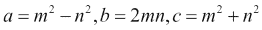
创建遮罩数组

遮罩数组可用于忽略丢失或无效的数据项。 numpy.ma模块中的MaskedArray类是ndarray的子类，带有遮罩。我们将使用 Lena 图像作为数据源，并假装其中一些数据已损坏。最后，我们将绘制原始图像，原始图像的对数值，遮罩数组及其对数值。

操作步骤

让我们创建被屏蔽的数组：

要创建一个遮罩数组，我们需要指定一个遮罩。创建一个随机遮罩，其值为0或1：
```
random_mask = np.random.randint(0, 2, size=lena.shape)
```

使用上一步中的遮罩，创建一个遮罩数组：

masked_array = np.ma.array(lena, mask=random_mask)

以下是此遮罩数组教程的完整代码：

from __future__ import print_function
import numpy as np
from scipy.misc import lena
import matplotlib.pyplot as plt

lena = lena()
random_mask = np.random.randint(0, 2, size=lena.shape)

plt.subplot(221)
plt.title("Original")
plt.imshow(lena)
plt.axis('off')

masked_array = np.ma.array(lena, mask=random_mask)
print(masked_array)
plt.subplot(222)
plt.title("Masked")
plt.imshow(masked_array)
plt.axis('off')
plt.subplot(223)
plt.title("Log")
plt.imshow(np.log(lena))
plt.axis('off')

plt.subplot(224)
plt.title("Log Masked")
plt.imshow(np.log(masked_array))
plt.axis('off')

plt.show()

这是显示结果图像的屏幕截图：

工作原理

我们对 NumPy 数组应用了随机的遮罩。这具有忽略对应于遮罩的数据的效果。您可以在numpy.ma 模块中找到一系列遮罩数组操作。在本教程中，我们仅演示了如何创建遮罩数组。

另见

numpy.ma模块的文档

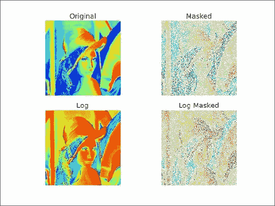
忽略负值和极值

当我们想忽略负值时，例如当取数组值的对数时，屏蔽的数组很有用。遮罩数组的另一个用例是排除极值。这基于极限值的上限和下限。

我们将把这些技术应用于股票价格数据。我们将跳过前面几章已经介绍的下载数据的步骤。

操作步骤

我们将使用包含负数的数组的对数：

创建一个数组，该数组包含可被三除的数字：

triples = np.arange(0, len(close), 3)
print("Triples", triples[:10], "...")

接下来，使用与价格数据数组大小相同的数组创建一个数组：

signs = np.ones(len(close))
print("Signs", signs[:10], "...")

借助您在第 2 章，“高级索引和数组概念”中学习的索引技巧，将每个第三个数字设置为负数。

signs[triples] = -1
print("Signs", signs[:10], "...")

最后，取该数组的对数：

ma_log = np.ma.log(close * signs)
print("Masked logs", ma_log[:10], "...")

这应该为AAPL打印以下输出：

Triples [ 0  3  6  9 12 15 18 21 24 27] ...
Signs [ 1\.  1\.  1\.  1\.  1\.  1\.  1\.  1\.  1\.  1.] ...
Signs [-1\.  1\.  1\. -1\.  1\.  1\. -1\.  1\.  1\. -1.] ...
Masked logs [-- 5.93655586575 5.95094223368 -- 5.97468290742 5.97510711452 --
 6.01674381162 5.97889061623 --] ...

让我们将极值定义为低于平均值的一个标准差，或高于平均值的一个标准差（这仅用于演示目的）。编写以下代码以屏蔽极值：

dev = close.std()
avg = close.mean()
inside = numpy.ma.masked_outside(close, avg - dev, avg + dev)
print("Inside", inside[:10], "...")

此代码显示前十个元素：

Inside [-- -- -- -- -- -- 409.429675172 410.240597855 -- --] ...

绘制原始价格数据，绘制对数后的数据，再次绘制指数，最后绘制基于标准差的遮罩后的数据。以下屏幕截图显示了结果（此运行）：

本教程的完整程序如下：

from __future__ import print_function
import numpy as np
from matplotlib.finance import quotes_historical_yahoo
from datetime import date
import matplotlib.pyplot as plt
def get_close(ticker):
   today = date.today()
   start = (today.year - 1, today.month, today.day)

   quotes = quotes_historical_yahoo(ticker, start, today)

   return np.array([q[4] for q in quotes])

close = get_close('AAPL')

triples = np.arange(0, len(close), 3)
print("Triples", triples[:10], "...")

signs = np.ones(len(close))
print("Signs", signs[:10], "...")

signs[triples] = -1
print("Signs", signs[:10], "...")

ma_log = np.ma.log(close * signs)
print("Masked logs", ma_log[:10], "...")

dev = close.std()
avg = close.mean()
inside = np.ma.masked_outside(close, avg - dev, avg + dev)
print("Inside", inside[:10], "...")

plt.subplot(311)
plt.title("Original")
plt.plot(close)

plt.subplot(312)
plt.title("Log Masked")
plt.plot(np.exp(ma_log))

plt.subplot(313)
plt.title("Not Extreme")
plt.plot(inside)

plt.tight_layout()
plt.show()

工作原理

numpy.ma模块中的函数掩盖了数组元素，我们认为这些元素是非法的。例如，log()和sqrt()函数不允许使用负值。屏蔽值类似于数据库和编程中的NULL或None值。具有屏蔽值的所有操作都将导致屏蔽值。

另见

numpy.ma模块的文档

使用`recarray`函数创建得分表

recarray类是ndarray的子类。这些数组可以像数据库中一样保存记录，具有不同的数据类型。例如，我们可以存储有关员工的记录，其中包含诸如薪水之类的数字数据和诸如员工姓名之类的字符串。

现代经济理论告诉我们，投资归结为优化风险和回报。风险是由对数回报的标准差表示的。另一方面，奖励由对数回报的平均值表示。我们可以拿出相对分数，高分意味着低风险和高回报。这只是理论上的，未经测试，所以不要太在意。我们将计算几只股票的得分，并将它们与股票代号一起使用 NumPy recarray()函数中的表格格式存储。

操作步骤

让我们从创建记录数组开始：

为每个记录创建一个包含符号，标准差得分，平均得分和总得分的记录数组：

weights = np.recarray((len(tickers),), dtype=[('symbol', np.str_, 16), 
    ('stdscore', float), ('mean', float), ('score', float)])

为了简单起见，请根据对数收益在循环中初始化得分：

for i, ticker in enumerate(tickers):
   close = get_close(ticker)
   logrets = np.diff(np.log(close))
   weights[i]['symbol'] = ticker
   weights[i]['mean'] = logrets.mean()
   weights[i]['stdscore'] = 1/logrets.std()
   weights[i]['score'] = 0

如您所见，我们可以使用在上一步中定义的字段名称来访问元素。

现在，我们有一些数字，但是它们很难相互比较。归一化分数，以便我们以后可以将它们合并。在这里，归一化意味着确保分数加起来为：
```
for key in ['mean', 'stdscore']:
    wsum = weights[key].sum()
    weights[key] = weights[key]/wsum
```

总体分数将只是中间分数的平均值。对总分上的记录进行排序以产生排名：

weights['score'] = (weights['stdscore'] + weights['mean'])/2
weights['score'].sort()

The following is the complete code for this example:

from __future__ import print_function
import numpy as np
from matplotlib.finance import quotes_historical_yahoo
from datetime import date

tickers = ['MRK', 'T', 'VZ']

def get_close(ticker):
   today = date.today()
   start = (today.year - 1, today.month, today.day)

   quotes = quotes_historical_yahoo(ticker, start, today)

   return np.array([q[4] for q in quotes])

weights = np.recarray((len(tickers),), dtype=[('symbol', np.str_, 16), 
   ('stdscore', float), ('mean', float), ('score', float)])

for i, ticker in enumerate(tickers):
   close = get_close(ticker)
   logrets = np.diff(np.log(close))
   weights[i]['symbol'] = ticker
   weights[i]['mean'] = logrets.mean()
   weights[i]['stdscore'] = 1/logrets.std()
   weights[i]['score'] = 0

for key in ['mean', 'stdscore']:
   wsum = weights[key].sum()
   weights[key] = weights[key]/wsum

weights['score'] = (weights['stdscore'] + weights['mean'])/2
weights['score'].sort()

for record in weights:
   print("%s,mean=%.4f,stdscore=%.4f,score=%.4f" % (record['symbol'], record['mean'], record['stdscore'], record['score']))

该程序产生以下输出：

MRK,mean=0.8185,stdscore=0.2938,score=0.2177
T,mean=0.0927,stdscore=0.3427,score=0.2262
VZ,mean=0.0888,stdscore=0.3636,score=0.5561

分数已归一化，因此值介于0和1之间，我们尝试从秘籍开始使用定义获得最佳收益和风险组合。根据输出，VZ得分最高，因此是最好的投资。当然，这只是一个 NumPy 演示，数据很少，所以不要认为这是推荐。

工作原理

我们计算了几只股票的得分，并将它们存储在recarray NumPy 对象中。这个数组使我们能够混合不同数据类型的数据，在这种情况下，是股票代码和数字得分。记录数组使我们可以将字段作为数组成员访问，例如arr.field。本教程介绍了记录数组的创建。您可以在numpy.recarray模块中找到更多与记录数组相关的功能。

另见

numpy.recarray模块的文档

七、性能分析和调试

在本章中，我们将介绍以下秘籍：

使用timeit进行性能分析
使用 IPython 进行分析
安装line_profiler
使用line_profiler分析代码
具有cProfile扩展名的性能分析代码
使用 IPython 进行调试
使用PuDB进行调试

简介

调试是从软件中查找和删除错误的行为。分析是指构建程序的概要文件，以便收集有关内存使用或时间复杂度的信息。分析和调试是开发人员生活中必不可少的活动。对于复杂的软件尤其如此。好消息是，许多工具可以为您提供帮助。我们将回顾 NumPy 用户中流行的技术。

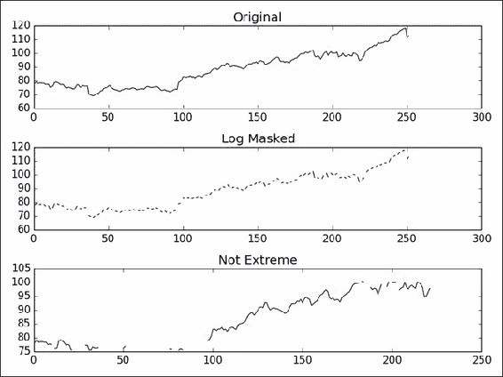
使用`timeit`进行性能分析

timeit是一个模块，可用于计时代码段。它是标准 Python 库的一部分。我们将使用几种数组大小对sort() NumPy 函数计时。经典的快速排序和归并排序算法的平均运行时间为O(N log N)，因此我们将尝试将这个模型拟合到结果。

操作步骤

我们将要求数组进行排序：

创建数组以排序包含随机整数值的各种大小：

times = np.array([])

for size in sizes:
    integers = np.random.random_integers (1, 10 ** 6, size)

要测量时间，请创建一个计时器，为其提供执行函数，并指定相关的导入。然后，排序 100 次以获取有关排序时间的数据：
```
def measure():
    timer = timeit.Timer('dosort()', 'from __main__ import dosort')
    return timer.timeit(10 ** 2)
```
通过一次乘以时间来构建测量时间数组：
```
times = np.append(times, measure())
```

将时间拟合为n log n的理论模型。由于我们将数组大小更改为 2 的幂，因此很容易：

fit = np.polyfit(sizes * powersOf2, times, 1)

以下是完整的计时代码：

import numpy as np
import timeit
import matplotlib.pyplot as plt

# This program measures the performance of the NumPy sort function
# and plots time vs array size.
integers = []

def dosort():
   integers.sort()

def measure():
   timer = timeit.Timer('dosort()', 'from __main__ import dosort')

   return timer.timeit(10 ** 2)

powersOf2 = np.arange(0, 19)
sizes = 2 ** powersOf2

times = np.array([])

for size in sizes:
   integers = np.random.random_integers(1, 10 ** 6, size)
   times = np.append(times, measure())

fit = np.polyfit(sizes * powersOf2, times, 1)
print(fit)
plt.title("Sort array sizes vs execution times")
plt.xlabel("Size")
plt.ylabel("(s)")
plt.semilogx(sizes, times, 'ro')
plt.semilogx(sizes, np.polyval(fit, sizes * powersOf2))
plt.grid()
plt.show()

以下屏幕截图显示了运行时间与数组大小的关系图：

工作原理

我们测量了sort() NumPy 函数的平均运行时间。此秘籍中使用了以下函数：

函数	描述
`random_integers()`	给定值和数组大小的范围时，此函数创建一个随机整数数组
`append()`	此函数将值附加到 NumPy 数组
`polyfit()`	此函数将数据拟合为给定阶数的多项式
`polyval()`	此函数计算多项式，并为给定的 `x`值返回相应的值
`semilogx()`	此函数使用对数刻度在 X 轴上绘制数据

另见

timeit的文档

使用 IPython 进行分析

在 IPython 中，我们可以使用timeit来分析代码的小片段。我们可以也分析较大的脚本。我们将展示两种方法。

操作步骤

首先，我们将介绍一个小片段：

以pylab模式启动 IPython：
```
$ ipython --pylab
```
创建一个包含 1000 个介于 0 到 1000 之间的整数值的数组：
```
In [1]: a = arange(1000)
```
测量在数组中搜索“所有问题的答案”（42）所花费的时间。是的，所有问题的答案都是 42。如果您不相信我，请阅读这个页面：
```
In [2]: %timeit searchsorted(a, 42)
100000 loops, best of 3: 7.58 us per loop
```

剖析以下小脚本，该小脚本可以反转包含随机值的大小可变的矩阵。 NumPy 矩阵的.I属性（即大写I）表示该矩阵的逆：

import numpy as np

def invert(n):
  a = np.matrix(np.random.rand(n, n))

  return a.I

sizes = 2 ** np.arange(0, 12)

for n in sizes:
  invert(n)

将此代码计时如下：

In [1]: %run -t invert_matrix.py

IPython CPU timings (estimated):
 User   :       6.08 s.
 System :       0.52 s.
Wall time:      19.26 s.

然后使用p选项对脚本进行配置：

In [2]: %run -p invert_matrix.py

852 function calls in 6.597 CPU seconds

   Ordered by: internal time

   ncalls  tottime  percall  cumtime  percall filename:lineno(function)
       12    3.228    0.269    3.228    0.269 {numpy.linalg.lapack_lite.dgesv}
       24    2.967    0.124    2.967    0.124 {numpy.core.multiarray._fastCopyAndTranspose}
       12    0.156    0.013    0.156    0.013 {method 'rand' of 'mtrand.RandomState' objects}
       12    0.087    0.007    0.087    0.007 {method 'copy' of 'numpy.ndarray' objects}
       12    0.069    0.006    0.069    0.006 {method 'astype' of 'numpy.ndarray' objects}
       12    0.025    0.002    6.304    0.525 linalg.py:404(inv)
       12    0.024    0.002    6.328    0.527 defmatrix.py:808(getI)
        1    0.017    0.017    6.596    6.596 invert_matrix.py:1(<module>)
       24    0.014    0.001    0.014    0.001 {numpy.core.multiarray.zeros}
       12    0.009    0.001    6.580    0.548 invert_matrix.py:3(invert)
       12    0.000    0.000    6.264    0.522 linalg.py:244(solve)
       12    0.000    0.000    0.014    0.001 numeric.py:1875(identity)
        1    0.000    0.000    6.597    6.597 {execfile}
       36    0.000    0.000    0.000    0.000 defmatrix.py:279(__array_finalize__)
       12    0.000    0.000    2.967    0.247 linalg.py:139(_fastCopyAndTranspose)
       24    0.000    0.000    0.087    0.004 defmatrix.py:233(__new__)
       12    0.000    0.000    0.000    0.000 linalg.py:99(_commonType)
       24    0.000    0.000    0.000    0.000 {method '__array_prepare__' of 'numpy.ndarray' objects}
       36    0.000    0.000    0.000    0.000 linalg.py:66(_makearray)
       36    0.000    0.000    0.000    0.000 {numpy.core.multiarray.array}
       12    0.000    0.000    0.000    0.000 {method 'view' of 'numpy.ndarray' objects}
       12    0.000    0.000    0.000    0.000 linalg.py:127(_to_native_byte_order)
        1    0.000    0.000    6.597    6.597 interactiveshell.py:2270(safe_execfile)

工作原理

我们通过分析器运行了上述 NumPy 代码。下表概述了分析器的输出：

函数	描述
`ncalls`	这是调用次数
`tottime`	这是一个函数花费的总时间
`percall`	这是每次通话所花费的时间，计算方法是将总时间除以通话次数
`cumtime`	这是在函数和由函数调用的函数（包括递归调用）上花费的累积时间

另见

IPython 魔术文档

安装`line_profiler`

line_profiler由 NumPy 的开发人员之一创建。此模块对 Python 代码进行逐行分析。我们将在此秘籍中描述必要的安装步骤。

准备

您可能需要安装setuptools。先前的秘籍中对此进行了介绍；如有必要，请参阅“另见”部分。为了安装开发版本，您将需要 Git。安装 Git 超出了本书的范围。

操作步骤

选择适合您的安装选项：

使用以下任一命令将line_profiler与easy_install一起安装：
```
$ easy_install line_profiler
$ pip install line_profiler
```
安装开发版本。

使用 Git 查看源代码：
```
$ git clone https://github.com/rkern/line_profiler
```
签出源代码后，按如下所示构建它：
```
$ python setup.py install
```

另见

第 1 章，“使用 IPython”中的“安装 IPython”

使用`line_profiler`分析代码

现在我们已经安装完毕，可以开始分析。

操作步骤

显然，我们将需要代码来分析：

编写以下代码，以自身乘以大小可变的随机矩阵。此外，线程将休眠几秒钟。使用@profile注解函数以进行概要分析：

import numpy as np
import time

@profile
def multiply(n):
  A = np.random.rand(n, n)
  time.sleep(np.random.randint(0, 2))
  return np.matrix(A) ** 2

for n in 2 ** np.arange(0, 10):
  multiply(n)

使用以下命令运行事件分析器：

$ kernprof.py -l -v mat_mult.py
Wrote profile results to mat_mult.py.lprof
Timer unit: 1e-06 s

File: mat_mult.py
Function: multiply at line 4
Total time: 3.19654 s

Line #      Hits         Time  Per Hit   % Time  Line Contents
==============================================================
 4                                           @profile
 5                                           def multiply(n):
 6        10        13461   1346.1      0.4     A = numpy.random.rand(n, n)
 7        10      3000689 300068.9     93.9     time.sleep(numpy.random.randint(0, 2))
 8        10       182386  18238.6      5.7     return numpy.matrix(A) ** 2

工作原理

@profile装饰器告诉line_profiler要分析哪些函数。下表说明了分析器的输出：

函数	描述
`Line #`	文件中的行号
`Hits`	执行该行的次数
`Time`	执行该行所花费的时间
`Per Hit`	执行该行所花费的平均时间
`% Time`	执行该行所花费的时间相对于执行所有行所花费的时间的百分比
`Line Contents`	该行的内容

另见

Github line_profiler项目页面

`cProfile`扩展和代码性能分析

cProfile是 Python 2.5 中引入的C扩展名。它可以用于确定性分析。确定性分析表示所获得的时间测量是精确的，并且不使用采样。这与统计分析相反，统计分析来自随机样本。我们将使用cProfile对一个小的 NumPy 程序进行分析，该程序会对具有随机值的数组进行转置。

操作步骤

同样，我们需要代码来配置：

编写以下transpose()函数以创建具有随机值的数组并将其转置：

def transpose(n):
  random_values = np.random.random((n, n))
  return random_values.T

运行分析器，并为其提供待分析函数：

cProfile.run('transpose (1000)')

可以在以下片段中找到本教程的完整代码：

import numpy as np
import cProfile

def transpose(n):
   random_values = np.random.random((n, n))
   return random_values.T

cProfile.run('transpose (1000)')

对于1000 x 1000的数组，我们得到以下输出：

4 function calls in 0.029 CPU seconds
 Ordered by: standard name
 ncalls  tottime  percall  cumtime  percall filename:lineno(function)
 1    0.001    0.001    0.029    0.029 <string>:1(<module>)
 1    0.000    0.000    0.028    0.028 cprofile_transpose.py:5(transpose)
 1    0.000    0.000    0.000    0.000 {method 'disable' of '_lsprof.Profiler' objects}
 1    0.028    0.028    0.028    0.028 {method 'random_sample' of 'mtrand.RandomState' objects}

输出中的列与 IPython 分析秘籍中看到的列相同。

另见

使用 IPython 进行调试

“如果调试是清除软件错误的过程，则编程必须是放入它们的过程。”

-- 荷兰计算机科学家 Edsger Dijkstra，1972 年图灵奖的获得者

调试是没人真正喜欢，但是掌握这些东西非常重要的东西之一。这可能需要几个小时，并且由于墨菲定律，您很可能没有时间。因此，重要的是要系统地了解您的工具。找到错误并实现修复后，您应该进行单元测试（如果该错误具有来自问题跟踪程序的相关 ID，我通常在末尾附加 ID 来命名测试）。这样，您至少不必再次进行调试。下一章将介绍单元测试。我们将调试以下错误代码。它尝试访问不存在的数组元素：

import numpy as np

a = np.arange(7)
print(a[8])

IPython 调试器充当普通的 Python pdb调试器；它添加了选项卡补全和语法突出显示等功能。

操作步骤

以下步骤说明了典型的调试会话：

启动 IPython Shell。通过发出以下命令在 IPython 中运行错误脚本：

In [1]: %run buggy.py
---------------------------------------------------------------------------
IndexError                                Traceback (most recent call last)
.../site-packages/IPython/utils/py3compat.pyc in execfile(fname, *where)
 173             else:
 174                 filename = fname
--> 175             __builtin__.execfile(filename, *where)

.../buggy.py in <module>()
 2
 3 a = numpy.arange(7)
----> 4 print a[8]

IndexError: index out of bounds

现在您的程序崩溃了，启动调试器。在发生错误的行上设置一个断点：
```
In [2]: %debug
> .../buggy.py(4)<module>()
 2 
 3 a = numpy.arange(7)
----> 4 print a[8]
```

使用list命令列出代码，或使用简写l：

ipdb> list
 1 import numpy as np
 2 
 3 a = np.arange(7)
----> 4 print(a[8])

现在，我们可以在调试器当前所在的行上求值任意代码：
```
ipdb> len(a)
7

ipdb> print(a)
[0 1 2 3 4 5 6]
```

调用栈是包含有关正在运行的程序的活动函数的信息的栈。使用bt命令查看调用栈：

ipdb> bt
 .../py3compat.py(175)execfile()
 171             if isinstance(fname, unicode):
 172                 filename = fname.encode(sys.getfilesystemencoding())
 173             else:
 174                 filename = fname
--> 175             __builtin__.execfile(filename, *where)

> .../buggy.py(4)<module>()
 0 print a[8]

向上移动调用栈：

ipdb> u
> .../site-packages/IPython/utils/py3compat.py(175)execfile()
 173             else:
 174                 filename = fname
--> 175             __builtin__.execfile(filename, *where)

下移调用栈：

ipdb> d
> .../buggy.py(4)<module>()
 2
 3 a = np.arange(7)
----> 4 print(a[8])

工作原理

在本教程中，您学习了如何使用 IPython 调试 NumPy 程序。我们设置一个断点并导航调用栈。使用了以下调试器命令：

函数	描述
`list`或 `l`	列出源代码
`bt`	显示调用栈
`u`	向上移动调用栈
`d`	下移调用栈

另见

使用 PuDB 进行调试

PuDB 是基于视觉的，全屏，基于控制台的 Python 调试器，易于安装。 PuDB 支持光标键和 vi 命令。如果需要，我们还可以将此调试器与 IPython 集成。

操作步骤

我们将从安装pudb开始：

要安装pudb，我们只需执行以下命令（或等效的pip命令）：

$ sudo easy_install pudb
$ pip install pudb
$ pip freeze|grep pudb
pudb==2014.1

让我们调试前面示例中的buggy程序。如下所示启动调试器：
```
$ python -m pudb buggy.py
```
以下屏幕截图显示了调试器的用户界面：

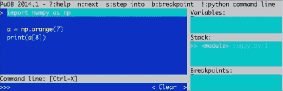
屏幕快照在顶部显示了最重要的调试命令。我们还可以看到正在调试的代码，变量，栈和定义的断点。键入q退出大多数菜单。键入n将调试器移至下一行。我们还可以使用光标键或 vi 的j和k键移动，例如，通过键入b设置断点。

另见

PyPi PuDB 页面

八、质量保证

“如果您对计算机撒谎，它将帮助您。”

-- Perry Farrar，ACM 通讯，第 28 卷

在本章中，我们将介绍以下秘籍：

安装 Pyflakes
使用 Pyflakes 执行静态分析
用 Pylint 分析代码
使用 Pychecker 执行静态分析
使用docstrings测试代码
编写单元测试
使用模拟测试代码
以 BDD 方式来测试

简介

与普遍的看法相反，质量保证与其说是发现错误，不如说是发现它们。我们将讨论两种提高代码质量，从而防止出现问题的方法。首先，我们将对已经存在的代码进行静态分析。然后，我们将讨论单元测试；这包括模拟和行为驱动开发（BDD）。

安装 Pyflakes

Pyflakes 是 Python 代码分析包。它可以分析代码并发现潜在的问题，例如：

未使用的导入
未使用的变量

准备

如有必要，请安装pip或easy_install。

操作步骤

选择以下之一来安装pyflakes：

使用pip命令安装 pyflakes：
```
$ sudo pip install pyflakes
```
使用easy_install命令安装 Pyflakes：
```
$ sudo easy_install pyflakes
```
这是在 Linux 上安装此包的两种方法：

Linux 包的名称也为pyflakes。例如，在 RedHat 上执行以下操作：
```
$ sudo yum install pyflakes
```
在 Debian/Ubuntu 上，命令如下：
```
$ sudo apt-get install pyflakes
```

另见

Pyflakes 主页

使用 Pyflakes 执行静态分析

我们将对 NumPy 代码库的一部分执行静态分析。为此，我们将使用 Git 签出代码。然后，我们将使用pyflakes对部分代码进行静态分析。

操作步骤

要检查 NumPy 代码中，我们需要 Git。安装 Git 超出了本书的范围：

用 Git 命令检索代码如下：
```
$ git clone git://github.com/numpy/numpy.git numpy
```
或者，从这里下载源档案。

上一步使用完整的 NumPy 代码创建一个numpy目录。转到此目录，并在其中运行以下命令：

$ pyflakes *.py
pavement.py:71: redefinition of unused 'md5' from line 69
pavement.py:88: redefinition of unused 'GIT_REVISION' from line 86
pavement.py:314: 'virtualenv' imported but unused
pavement.py:315: local variable 'e' is assigned to but never used
pavement.py:380: local variable 'sdir' is assigned to but never used
pavement.py:381: local variable 'bdir' is assigned to but never used
pavement.py:536: local variable 'st' is assigned to but never used
setup.py:21: 're' imported but unused
setup.py:27: redefinition of unused 'builtins' from line 25
setup.py:124: redefinition of unused 'GIT_REVISION' from line 118
setupegg.py:17: 'setup' imported but unused
setupscons.py:61: 'numpy' imported but unused
setupscons.py:64: 'numscons' imported but unused
setupsconsegg.py:6: 'setup' imported but unused

这将对代码样式进行分析，并检查当前目录中所有 Python 脚本中的 PEP-8 违规情况。如果愿意，还可以分析单个文件。

工作原理

正如您所见，分析代码样式并使用 Pyflakes 查找违反 PEP-8 的行为非常简单。另一个优点是速度。但是，Pyflakes 报告的错误类型的数量是有限的。

使用 Pylint 分析代码

Pylint 是另一个由 Logilab 创建的开源静态分析器。 Pylint 比 Pyflakes 更复杂；它允许更多的自定义和代码检查。但是，它比 Pyflakes 慢。有关更多信息，请参见手册。

在本秘籍中，我们再次从 Git 存储库下载 NumPy 代码-为简便起见，省略了此步骤。

准备

您可以从源代码发行版中安装 Pylint。但是，有很多依赖项，因此最好使用easy_install或pip进行安装。安装命令如下：

$ easy_install pylint
$ sudo pip install pylint

操作步骤

我们将再次从 NumPy 代码库的顶部目录进行分析。注意，我们得到了更多的输出。实际上，Pylint 打印了太多文本，因此在这里大部分都必须省略：

$ pylint *.py
No config file found, using default configuration
************* Module pavement
C: 60: Line too long (81/80)
C:139: Line too long (81/80)
...
W: 50: TODO
W:168: XXX: find out which env variable is necessary to avoid the pb with python
W: 71: Reimport 'md5' (imported line 143)
F: 73: Unable to import 'paver'
F: 74: Unable to import 'paver.easy'
C: 79: Invalid name "setup_py" (should match (([A-Z_][A-Z0-9_]*)|(__.*__))$)
F: 86: Unable to import 'numpy.version'
E: 86: No name 'version' in module 'numpy'
C:149: Operator not followed by a space
if sys.platform =="darwin":
 ^^
C:202:prepare_nsis_script: Missing docstring
W:228:bdist_superpack: Redefining name 'options' from outer scope (line 74)
C:231:bdist_superpack.copy_bdist: Missing docstring
W:275:bdist_wininst_nosse: Redefining name 'options' from outer scope (line 74)

工作原理

Pylint 默认输出原始文本；但是我们可以根据需要请求 HTML 输出。消息具有以下格式：

MESSAGE_TYPE: LINE_NUM:[OBJECT:] MESSAGE

消息类型可以是以下之一：

[R]：这意味着建议进行重构
[C]：这意味着存在违反代码风格的情况
[W]：用于警告小问题
[E]：用于错误或潜在的错误
[F]：这表明发生致命错误，阻止了进一步的分析

另见

使用 Pyflakes 执行静态分析

使用 Pychecker 执行静态分析

Pychecker 是一个古老的静态分析工具。它不是十分活跃的开发工具，但它在此提到的速度又足够好。在编写本书时，最新版本是 0.8.19，最近一次更新是在 2011 年。Pychecker 尝试导入每个模块并对其进行处理。然后，它搜索诸如传递不正确数量的参数，使用不存在的方法传递不正确的格式字符串以及其他问题之类的问题。在本秘籍中，我们将再次分析代码，但是这次使用 Pychecker。

操作步骤

从 Sourceforge 下载tar.gz。解压缩源归档文件并运行以下命令：

$ python setup.py install

或者，使用pip安装 Pychecker：

$ sudo pip install http://sourceforge.net/projects/pychecker/files/pychecker/0.8.19/pychecker-0.8.19.tar.gz/download

分析代码，就像先前的秘籍一样。我们需要的命令如下：

$ pychecker *.py
...
Warnings...

...

setup.py:21: Imported module (re) not used
setup.py:27: Module (builtins) re-imported

...

使用文档字符串测试代码

Doctests 是注释字符串，它们嵌入在类似交互式会话的 Python 代码中。这些字符串可用于测试某些假设或仅提供示例。我们需要使用doctest模块来运行这些测试。

让我们写一个简单的示例，该示例应该计算阶乘，但不涵盖所有可能的边界条件。换句话说，某些测试将失败。

操作步骤

用将通过的测试和将失败的另一个测试编写docstring。 docstring文本应类似于在 Python shell 中通常看到的文本：

"""
Test for the factorial of 3 that should pass.
>>> factorial(3)
6

Test for the factorial of 0 that should fail.
>>> factorial(0)
1
"""

编写以下 NumPy 代码：
```
return np.arange(1, n+1).cumprod()[-1]
```
我们希望这段代码有时会故意失败。它将创建一个序列号数组，计算该数组的累积乘积，并返回最后一个元素。

使用doctest模块运行测试：

doctest.testmod()

以下是本书代码包中docstringtest.py文件的完整测试示例代码：

import numpy as np
import doctest

def factorial(n):
   """
   Test for the factorial of 3 that should pass.
   >>> factorial(3)
   6

   Test for the factorial of 0 that should fail.
   >>> factorial(0)
   1
   """
   return np.arange(1, n+1).cumprod()[-1]

doctest.testmod()

我们可以使用-v选项获得详细的输出，如下所示：

$ python docstringtest.py -v
Trying:
 factorial(3)
Expecting:
 6
ok
Trying:
 factorial(0)
Expecting:
 1
**********************************************************************
File "docstringtest.py", line 11, in __main__.factorial
Failed example:
 factorial(0)
Exception raised:
 Traceback (most recent call last):
 File ".../doctest.py", line 1253, in __run
 compileflags, 1) in test.globs
 File "<doctest __main__.factorial[1]>", line 1, in <module>
 factorial(0)
 File "docstringtest.py", line 14, in factorial
 return numpy.arange(1, n+1).cumprod()[-1]
 IndexError: index out of bounds
1 items had no tests:
 __main__
**********************************************************************
1 items had failures:
 1 of   2 in __main__.factorial
2 tests in 2 items.
1 passed and 1 failed.
***Test Failed*** 1 failures.

工作原理

如您所见，我们没有考虑零和负数。实际上，由于数组为空，我们出现了index out of bounds错误。当然，这很容易解决，我们将在下一个教程中进行。

另见

doctest官方文档

编写单元测试

测试驱动开发（TDD）是本世纪软件开发诞生的最好的事情。 TDD 的最重要方面之一是，几乎把重点放在单元测试上。

注意

TDD 方法使用所谓的测试优先方法，在此方法中，我们首先编写一个失败的测试，然后编写相应的代码以通过测试。测试应记录开发人员的意图，但要比功能设计的水平低。一组测试通过降低回归概率来增加置信度，并促进重构。

单元测试是自动测试，通常测试一小段代码，通常是一个函数或方法。 Python 具有用于单元测试的 PyUnit API。作为 NumPy 的用户，我们也可以使用numpy.testing模块中的便捷函数。顾名思义，该模块专用于测试。

操作步骤

让我们编写一些代码进行测试：

首先编写以下factorial()函数：

def factorial(n):
  if n == 0:
    return 1

  if n < 0:
    raise ValueError, "Don't be so negative"

  return np.arange(1, n+1).cumprod()

该代码与前面的秘籍中的代码相同，但是我们添加了一些边界条件检查。

让我们写一个类；此类将包含单元测试。它从unittest模块扩展了TestCase类，是 Python 标准测试的一部分。我们通过调用factorial()函数并运行以下代码来运行测试：

一个正数-幸福的道路！
边界条件等于0

负数，这将导致错误：

class FactorialTest(unittest.TestCase):
    def test_factorial(self):
      #Test for the factorial of 3 that should pass.
      self.assertEqual(6, factorial(3)[-1])
      np.testing.assert_equal(np.array([1, 2, 6]), factorial(3))

    def test_zero(self):
      #Test for the factorial of 0 that should pass.
      self.assertEqual(1, factorial(0))

    def test_negative(self):
      #Test for the factorial of negative numbers that should fail.
      # It should throw a ValueError, but we expect IndexError
      self.assertRaises(IndexError, factorial(-10))

factorial()函数和整个单元测试的代码如下：

import numpy as np
import unittest

def factorial(n):
   if n == 0:
      return 1

   if n < 0:
      raise ValueError, "Don't be so negative"

   return np.arange(1, n+1).cumprod()

class FactorialTest(unittest.TestCase):
   def test_factorial(self):
      #Test for the factorial of 3 that should pass.
      self.assertEqual(6, factorial(3)[-1])
      np.testing.assert_equal(np.array([1, 2, 6]), factorial(3))

   def test_zero(self):
      #Test for the factorial of 0 that should pass.
      self.assertEqual(1, factorial(0))

   def test_negative(self):
      #Test for the factorial of negative numbers that should fail.
      # It should throw a ValueError, but we expect IndexError
      self.assertRaises(IndexError, factorial(-10))

if __name__ == '__main__':
    unittest.main()

负数测试失败，如以下输出所示：

.E.
======================================================================
ERROR: test_negative (__main__.FactorialTest)
----------------------------------------------------------------------
Traceback (most recent call last):
 File "unit_test.py", line 26, in test_negative
 self.assertRaises(IndexError, factorial(-10))
 File "unit_test.py", line 9, in factorial
 raise ValueError, "Don't be so negative"
ValueError: Don't be so negative

----------------------------------------------------------------------
Ran 3 tests in 0.001s

FAILED (errors=1)

工作原理

我们看到了如何使用标准unittest Python 模块实现简单的单元测试。我们编写了一个测试类，该类从unittest模块扩展了TestCase类。以下函数用于执行各种测试：

函数	描述
`numpy.testing.assert_equal()`	测试两个 NumPy 数组是否相等
`unittest.assertEqual()`	测试两个值是否相等
`unittest.assertRaises()`	测试是否引发异常

testing NumPy 包具有许多我们应该了解的测试函数，如下所示：

函数	描述
`assert_almost_equal()`	如果两个数字不等于指定的精度，则此函数引发异常
`assert_approx_equal()`	如果两个数字在一定意义上不相等，则此函数引发异常
`assert_array_almost_equal()`	如果两个数组不等于指定的精度，此函数会引发异常
`assert_array_equal()`	如果两个数组不相等，则此函数引发异常
`assert_array_less()`	如果两个数组的形状不同，并且此函数引发异常，则第一个数组的元素严格小于第二个数组的元素
`assert_raises()`	如果使用定义的参数调用的可调用对象未引发指定的异常，则此函数将失败
`assert_warns()`	如果未抛出指定的警告，则此函数失败
`assert_string_equal()`	此函数断言两个字符串相等

使用模拟测试代码

模拟是用来代替真实对象的对象，目的是测试真实对象的部分行为。如果您看过电影《身体抢夺者》，您可能已经对基本概念有所了解。一般来说，仅在被测试的真实对象的创建成本很高（例如数据库连接）或测试可能产生不良副作用时才有用。例如，我们可能不想写入文件系统或数据库。

在此秘籍中，我们将测试一个核反应堆，当然不是真正的反应堆！此类核反应堆执行阶乘计算，从理论上讲，它可能导致连锁反应，进而导致核灾难。我们将使用mock包通过模拟来模拟阶乘计算。

操作步骤

首先，我们将安装mock包；之后，我们将创建一个模拟并测试一段代码：

要安装mock包，请执行以下命令：
```
$ sudo easy_install mock
```
核反应堆类有一个do_work()方法，该方法调用了我们要模拟的危险的factorial()方法。创建一个模拟，如下所示：
```
reactor.factorial = MagicMock(return_value=6)
```
这样可以确保模拟返回值6。

我们可以通过多种方式检查模拟的行为，然后从中检查真实对象的行为。例如，断言使用正确的参数调用了潜在爆炸性的factorial()方法，如下所示：

reactor.factorial.assert_called_with(3, "mocked")

带有模拟的完整测试代码如下：

from __future__ import print_function
from mock import MagicMock
import numpy as np
import unittest

class NuclearReactor():
   def __init__(self, n):
      self.n = n

   def do_work(self, msg):
      print("Working")

      return self.factorial(self.n, msg)

   def factorial(self, n, msg):
      print(msg)

      if n == 0:
         return 1

      if n < 0:
         raise ValueError, "Core meltdown"

      return np.arange(1, n+1).cumprod()

class NuclearReactorTest(unittest.TestCase):
   def test_called(self):
      reactor = NuclearReactor(3)
      reactor.factorial = MagicMock(return_value=6)
      result = reactor.do_work("mocked")
      self.assertEqual(6, result)
      reactor.factorial.assert_called_with(3, "mocked")

   def test_unmocked(self):
      reactor = NuclearReactor(3)
      reactor.factorial(3, "unmocked")
      np.testing.assert_raises(ValueError)

if __name__ == '__main__':
    unittest.main()

我们将一个字符串传递给factorial()方法，以显示带有模拟的代码不会执行实际的代码。该单元测试的工作方式与上一秘籍中的单元测试相同。这里的第二项测试不测试任何内容。第二个测试的目的只是演示，如果我们在没有模拟的情况下执行真实代码，会发生什么。

测试的输出如下：

Working
.unmocked
.
----------------------------------------------------------------------
Ran 2 tests in 0.000s

OK

工作原理

模拟没有任何行为。他们就像外星人的克隆人，假装是真实的人。只能比外星人傻—外星人克隆人无法告诉您被替换的真实人物的生日。我们需要设置它们以适当的方式进行响应。例如，在此示例中，模拟返回6 。我们可以记录模拟发生了什么，被调用了多少次以及使用了哪些参数。

另见

Mock 包主页

以 BDD 方式来测试

BDD（行为驱动开发）是您可能遇到的另一个热门缩写。在 BDD 中，我们首先根据某些约定和规则定义（英语）被测系统的预期行为。在本秘籍中，我们将看到这些约定的示例。

这种方法背后的想法是，我们可以让可能无法编程或编写测试大部分内容的人员参加。这些人编写的功能采用句子的形式，包括多个步骤。每个步骤或多或少都是我们可以编写的单元测试，例如，使用 NumPy。有许多 Python BDD 框架。在本秘籍中，我们使用 Lettuce 来测试阶乘函数。

操作步骤

在本节中，您将学习如何安装 Lettuce，设置测试以及编写测试规范：

要安装 Lettuce，请运行以下命令之一：

$ pip install lettuce
$ sudo easy_install lettuce

Lettuce 需要特殊的目录结构进行测试。在tests目录中，我们将有一个名为features的目录，其中包含factorial.feature文件，以及steps.py文件中的功能说明和测试代码：
```
./tests:
features

./tests/features:
factorial.feature	steps.py
```

提出业务需求是一项艰巨的工作。以易于测试的方式将其全部写下来更加困难。幸运的是，这些秘籍的要求非常简单-我们只需写下不同的输入值和预期的输出。我们在Given，When和Then部分中有不同的方案，它们对应于不同的测试步骤。为阶乘函数定义以下三种方案：

Feature: Compute factorial

    Scenario: Factorial of 0
      Given I have the number 0 
      When I compute its factorial 
      Then I see the number 1

    Scenario: Factorial of 1
      Given I have the number 1 
      When I compute its factorial 
      Then I see the number 1

    Scenario: Factorial of 3
      Given I have the number 3 
      When I compute its factorial 
      Then I see the number 1, 2, 6

我们将定义与场景步骤相对应的方法。要特别注意用于注释方法的文本。它与业务场景文件中的文本匹配，并且我们使用正则表达式获取输入参数。在前两个方案中，我们匹配数字，在最后一个方案中，我们匹配任何文本。 fromstring() NumPy 函数用于从 NumPy 数组创建字符串，字符串中使用整数数据类型和逗号分隔符。以下代码测试了我们的方案：

from lettuce import *
import numpy as np

@step('I have the number (\d+)')
def have_the_number(step, number):
    world.number = int(number)

@step('I compute its factorial')
def compute_its_factorial(step):
    world.number = factorial(world.number)

@step('I see the number (.*)')
def check_number(step, expected):
    expected = np.fromstring(expected, dtype=int, sep=',')
    np.testing.assert_equal(world.number, expected, \
        "Got %s" % world.number)

def factorial(n):
   if n == 0:
      return 1

   if n < 0:
      raise ValueError, "Core meltdown"

   return np.arange(1, n+1).cumprod()

要运行测试，请转到tests目录，然后键入以下命令：

$ lettuce

Feature: Compute factorial        # features/factorial.feature:1

 Scenario: Factorial of 0        # features/factorial.feature:3
 Given I have the number 0     # features/steps.py:5
 When I compute its factorial  # features/steps.py:9
 Then I see the number 1       # features/steps.py:13

 Scenario: Factorial of 1        # features/factorial.feature:8
 Given I have the number 1     # features/steps.py:5
 When I compute its factorial  # features/steps.py:9
 Then I see the number 1       # features/steps.py:13

 Scenario: Factorial of 3        # features/factorial.feature:13
 Given I have the number 3     # features/steps.py:5
 When I compute its factorial  # features/steps.py:9
 Then I see the number 1, 2, 6 # features/steps.py:13

1 feature (1 passed)
3 scenarios (3 passed)
9 steps (9 passed)

工作原理

我们定义了具有三个方案和相应步骤的函数。我们使用 NumPy 的测试函数来测试不同步骤，并使用fromstring()函数从规格文本创建 NumPy 数组。

另见

Lettuce 文档

九、使用 Cython 加速代码

在本章中，我们将介绍以下秘籍：

安装 Cython
构建 HelloWorld 程序
将 Cython 与 NumPy 结合使用
调用 C 函数
分析 Cython 代码
用 Cython 近似阶乘

简介

Cython 是基于 Python 的相对年轻的编程语言。它允许编码人员将 C 的速度与 Python 的功能混合在一起。与 Python 的区别在于我们可以选择声明静态类型。许多编程语言（例如 C）具有静态类型，这意味着我们必须告诉 C 变量的类型，函数参数和返回值类型。另一个区别是 C 是一种编译语言，而 Python 是一种解释语言。根据经验，可以说 C 比 Python 更快，但灵活性更低。通过 Cython 代码，我们可以生成 C 或 C++ 代码。之后，我们可以将生成的代码编译为 Python 扩展模块。

在本章中，您将学习 Cython。我们将获得一些与 NumPy 一起运行的简单 Cython 程序。另外，我们将介绍 Cython 代码。

安装 Cython

为了使用 Cython，我们需要安装它。 Enthought Canopy，Anaconda 和 Sage 发行版包括 Cython。有关更多信息，请参见这里，这里和这里。我们将不在这里讨论如何安装这些发行版。显然，我们需要一个 C 编译器来编译生成的 C 代码。在某些操作系统（例如 Linux）上，编译器将已经存在。在本秘籍中，我们将假定您已经安装了编译器。

操作步骤

我们可以使用以下任何一种方法来安装 Cython：

通过执行以下步骤从源存档中安装 Cython ：
- 下载源归档文件。
- 打开包装。
- 使用cd命令浏览到目录。
- 运行以下命令：
```
$ python setup.py install
```
使用以下任一命令从 PyPI 存储库安装 Cython：
```
$ easy_install cython
$ sudo pip install cython
```
使用非官方 Windows 安装程序，在 Windows 上安装 Cython。

另见

相关的 Cython 在线文档

构建 HelloWorld 程序

与编程语言的传统一样，我们将从 HelloWorld 示例开始。与 Python 不同，我们需要编译 Cython 代码。我们从.pyx文件开始，然后从中生成 C 代码。可以编译此.c文件，然后将其导入 Python 程序中。

操作步骤

本节介绍如何构建 Cython HelloWorld 程序：

首先，编写一些非常简单的代码以显示Hello World。这只是普通的 Python 代码，但文件具有pyx扩展名：
```
def say_hello():
  print "Hello World!"
```

创建一个名为setup.py的文件来帮助构建 Cython 代码：

from distutils.core import setup
from distutils.extension import Extension
from Cython.Distutils import build_ext

ext_modules = [Extension("hello", ["hello.pyx"])]

setup(
        name = 'Hello world app',
        cmdclass = {'build_ext': build_ext},
        ext_modules = ext_modules
     )

如您所见，我们在上一步中指定了文件，并为应用命名。

使用以下命令进行构建：
```
$ python setup.py build_ext --inplace
```
这将生成 C 代码，将其编译为您的平台，并产生以下输出：
```
running build_ext
cythoning hello.pyx to hello.c
building 'hello' extension
creating build
```
现在，我们可以使用以下语句导入模块：
```
from hello import say_hello
```

工作原理

在此秘籍中，我们创建了一个传统的 HelloWorld 示例。 Cython 是一种编译语言，因此我们需要编译代码。我们编写了一个包含Hello World代码的.pyx文件和一个用于生成和构建 C 代码的setup.py文件。

另见

相关的 Cython 的在线文档

将 Cython 与 NumPy 结合使用

我们可以集成 Cython 和 NumPy 代码，就像可以集成 Cython 和 Python 代码一样。让我们来看一个示例，该示例分析股票的上涨天数（股票收盘价高于前一日的天数）的比率。我们将应用二项式比值置信度的公式。您可以参考这里了解更多信息。以下公式说明该比率的重要性：

式中，p是概率，n是观察数。

操作步骤

本节通过以下步骤介绍如何将 Cython 与 NumPy 结合使用：

编写一个.pyx文件，其中包含一个函数，该函数可计算上升天数的比率和相关的置信度。首先，此函数计算价格之间的差异。然后，它计算出正差的数量，从而得出上升天数的比率。最后，在引言中的维基百科页面上应用置信度公式：
```
import numpy as np

def pos_confidence(numbers):
   diffs = np.diff(numbers)
   n = float(len(diffs))
   p = len(diffs[diffs > 0])/n
   confidence = np.sqrt(p * (1 - p)/ n)

   return (p, confidence)
```

使用上一个示例中的setup.py文件作为模板。更改明显的内容，例如.pyx文件的名称：

from distutils.core import setup
from distutils.extension import Extension
from Cython.Distutils import build_ext

ext_modules = [Extension("binomial_proportion", ["binomial_proportion.pyx"])]

setup(
        name = 'Binomial proportion app',
        cmdclass = {'build_ext': build_ext},
        ext_modules = ext_modules
     )

我们现在可以建立；有关更多详细信息，请参见前面的秘籍。

构建后，通过导入使用上一步中的 Cython 模块。我们将编写一个 Python 程序，使用matplotlib下载股价数据。然后我们将confidence()函数应用于收盘价：

from matplotlib.finance import quotes_historical_yahoo
from datetime import date
import numpy
import sys
from binomial_proportion import pos_confidence

#1\. Get close prices.
today = date.today()
start = (today.year - 1, today.month, today.day)

quotes = quotes_historical_yahoo(sys.argv[1], start, today)
close =  numpy.array([q[4] for q in quotes])
print pos_confidence(close)

AAPL程序的输出如下：

(0.56746031746031744, 0.031209043355655924)

工作原理

我们计算了APL股价上涨的可能性和相应的置信度。我们通过创建 Cython 模块，将 NumPy 代码放入.pyx文件中，并按照上一教程中的步骤进行构建。最后，我们导入并使用了 Cython 模块。

另见

有关 Cython 的在线文档

调用 C 函数

我们可以从 Cython 调用 C 函数。在此示例中，我们调用 C log()函数。此函数仅适用于单个数字。请记住，NumPy log()函数也可以与数组一起使用。我们将计算股票价格的所谓对数回报。

操作步骤

我们首先编写一些 Cython 代码：

首先，从libc命名空间导入 C 的log()函数。然后，将此函数应用于for循环中的数字。最后，使用 NumPy diff()函数在第二步中获取对数值之间的一阶差：
```
from libc.math cimport log
import numpy as np

def logrets(numbers):
   logs = [log(x) for x in numbers] 
   return np.diff(logs)
```
先前的秘籍中已经介绍了架构。我们只需要更改setup.py文件中的某些值。

再次使用 matplotlib 下载股价数据。应用您刚刚在价格上创建的 Cython logrets()函数并绘制结果：

from matplotlib.finance import quotes_historical_yahoo
from datetime import date
import numpy as np
from log_returns import logrets
import matplotlib.pyplot as plt

today = date.today()
start = (today.year - 1, today.month, today.day)

quotes = quotes_historical_yahoo('AAPL', start, today)
close =  np.array([q[4] for q in quotes])
plt.plot(logrets(close))
plt.title('Logreturns of AAPL for the previous year')
plt.xlabel('Days')
plt.ylabel('Log returns')
plt.grid()
plt.show()

的AAPL对数回报结果图类似于以下屏幕截图所示：

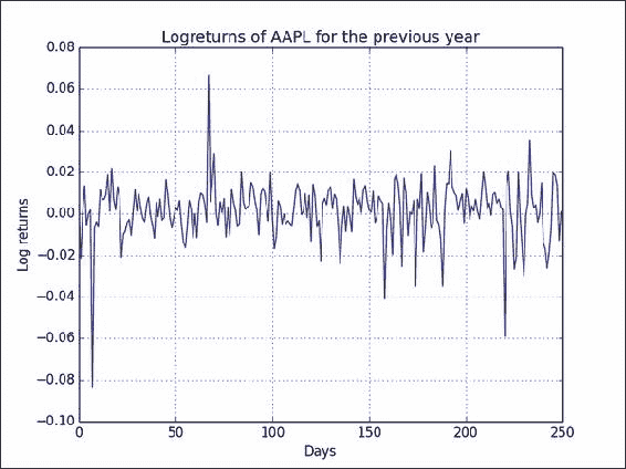
工作原理

我们从 Cython 代码中调用了 C log()函数。该函数与 NumPy 函数一起用于计算股票的对数收益。这样，我们可以创建自己的包含便利函数的专用 API。令人高兴的是，我们的代码应该或多或少地像 Python 代码一样，以与 C 代码差不多的速度执行。

另见

相关的 Cython 在线文档位于

分析 Cython 代码

我们将使用以下公式对 Cython 和 NumPy 代码进行剖析，这些代码试图近似于欧拉常数：

有关更多背景信息，请参见。

操作步骤

本节演示如何通过以下步骤来分析 Cython 代码：

对于e的 NumPy 近似值，请按照下列步骤操作：

首先，我们将创建一个1到n的数组（在我们的示例中n是40）。

然后，我们将计算该数组的累积乘积，该乘积恰好是阶乘。在那之后，我们采取阶乘的倒数。最后，我们从维基百科页面应用公式。最后，我们放入标准配置代码，为我们提供以下程序：

from __future__ import print_function
import numpy as np
import cProfile
import pstats

def approx_e(n=40, display=False):
   # array of [1, 2, ... n-1]
   arr = np.arange(1, n)

   # calculate the factorials and convert to floats
   arr = arr.cumprod().astype(float)

   # reciprocal 1/n
   arr = np.reciprocal(arr)

   if display:
    print(1 + arr.sum())

# Repeat multiple times because NumPy is so fast
def run(repeat=2000):
    for i in range(repeat):
        approx_e()

cProfile.runctx("run()", globals(), locals(), "Profile.prof")

s = pstats.Stats("Profile.prof")
s.strip_dirs().sort_stats("time").print_stats()

approx_e(display=True)

以下代码段显示了e的近似值的分析输出和结果。有关概要分析输出的更多信息，请参见第 7 章，“分析和调试”。

 8004 function calls in 0.016 seconds

 Ordered by: internal time

 ncalls  tottime  percall  cumtime  percall filename:lineno(function)
 2000    0.007    0.000    0.015    0.000 numpy_approxe.py:6(approx_e)
 2000    0.004    0.000    0.004    0.000 {method 'cumprod' of 'numpy.ndarray' objects}
 2000    0.002    0.000    0.002    0.000 {numpy.core.multiarray.arange}
 2000    0.002    0.000    0.002    0.000 {method 'astype' of 'numpy.ndarray' objects}
 1    0.001    0.001    0.016    0.016 numpy_approxe.py:20(run)
 1    0.000    0.000    0.000    0.000 {range}
 1    0.000    0.000    0.016    0.016 <string>:1(<module>)
 1    0.000    0.000    0.000    0.000 {method 'disable' of '_lsprof.Profiler' objects}

2.71828182846

Cython 代码使用与上一步所示相同的算法，但是实现方式不同。便利函数较少，实际上我们现在需要一个for循环。另外，我们需要为某些变量指定类型。 .pyx文件的代码如下所示：

def approx_e(int n=40, display=False):
    cdef double sum = 0.
    cdef double factorial = 1.
    cdef int k

    for k in xrange(1,n+1):
        factorial *= k
        sum += 1/factorial

    if display:
        print(1 + sum)

以下 Python 程序导入 Cython 模块并进行一些分析：

import pstats
import cProfile
import pyximport
pyximport.install()

import approxe

# Repeat multiple times because Cython is so fast
def run(repeat=2000):
    for i in range(repeat):
        approxe.approx_e()

cProfile.runctx("run()", globals(), locals(), "Profile.prof")

s = pstats.Stats("Profile.prof")
s.strip_dirs().sort_stats("time").print_stats()

approxe.approx_e(display=True)

这是 Cython 代码的分析输出：

 2004 function calls in 0.001 seconds

 Ordered by: internal time

 ncalls  tottime  percall  cumtime  percall filename:lineno(function)
 2000    0.001    0.000    0.001    0.000 {approxe.approx_e}
 1    0.000    0.000    0.001    0.001 cython_profile.py:9(run)
 1    0.000    0.000    0.000    0.000 {range}
 1    0.000    0.000    0.001    0.001 <string>:1(<module>)
 1    0.000    0.000    0.000    0.000 {method 'disable' of '_lsprof.Profiler' objects}

2.71828182846

工作原理

我们分析了 NumPy 和 Cython 代码。 NumPy 已针对速度进行了优化，因此 NumPy 和 Cython 程序都是高性能程序，我们对此不会感到惊讶。但是，当比较 2,000 次近似代码的总时间时，我们意识到 NumPy 需要 0.016 秒，而 Cython 仅需要 0.001 秒。显然，实际时间取决于硬件，操作系统和其他因素，例如计算机上运行的其他进程。同样，提速取决于代码类型，但我希望您同意，根据经验，Cython 代码会更快。

另见

相关的 Cython 在线文档

Cython 的近似阶乘

最后一个示例是 Cython 的近似阶乘。我们将使用两种近似方法。首先，我们将应用斯特林近似方法。斯特林近似的公式如下：

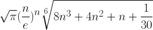
其次，我们将使用 Ramanujan 的近似值，并使用以下公式：

操作步骤

本节介绍如何使用 Cython 近似阶乘。您可能还记得，在本秘籍中，我们使用在 Cython 中可选的类型。从理论上讲，声明静态类型应加快速度。静态类型化提供了一些有趣的挑战，这些挑战在编写 Python 代码时可能不会遇到，但请不要担心。我们将尝试使其简单：

除了将函数参数和一个局部变量声明为ndarray数组外，我们将编写的 Cython 代码类似于常规的 Python 代码。为了使静态类型起作用，我们需要cimport NumPy。另外，我们必须使用cdef关键字声明局部变量的类型：

import numpy
cimport numpy

def ramanujan_factorial(numpy.ndarray n):
   sqrt_pi = numpy.sqrt(numpy.pi, dtype=numpy.float64)
   cdef numpy.ndarray root = (8 * n + 4) * n + 1 
   root = root * n + 1/30.
   root = root ** (1/6.)
   return sqrt_pi * calc_eton(n) * root

def stirling_factorial(numpy.ndarray n):
    return numpy.sqrt(2 * numpy.pi * n) * calc_eton(n)

def calc_eton(numpy.ndarray n):
    return (n/numpy.e) ** n

如先前的教程所示，构建需要我们创建一个setup.py文件，但是现在我们通过调用get_include()函数来包含与 NumPy 相关的目录。通过此修订，setup.py文件具有以下内容：

from distutils.core import setup
from distutils.extension import Extension
from Cython.Distutils import build_ext
import numpy

ext_modules = [Extension("factorial", ["factorial.pyx"], include_dirs = [numpy.get_include()])] 

setup(
        name = 'Factorial app',
        cmdclass = {'build_ext': build_ext},
        ext_modules = ext_modules
     )

绘制两种近似方法的相对误差。像我们在整本书中所做的那样，将使用 NumPy cumprod()函数计算相对于阶乘值的误差：

from factorial import ramanujan_factorial
from factorial import stirling_factorial
import numpy as np
import matplotlib.pyplot as plt

N = 50
numbers = np.arange(1, N)
factorials = np.cumprod(numbers, dtype=float)

def error(approximations):
   return (factorials - approximations)/factorials

plt.plot(error(ramanujan_factorial(numbers)), 'b-', label='Ramanujan')
plt.plot(error(stirling_factorial(numbers)), 'ro', label='Stirling')
plt.title('Factorial approximation relative errors')
plt.xlabel('n')
plt.ylabel('Relative error')
plt.grid()
plt.legend(loc='best')
plt.show()

下图显示了 Ramanujan 近似值（点）和 Stirling 近似值（线）的相对误差：

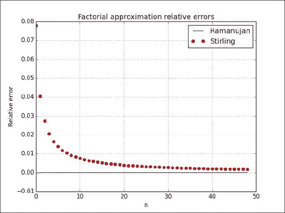
工作原理

在此示例中，我们看到了 Cython 静态类型的演示。该秘籍的主要成分如下：

cimport，它导入 C 声明
包含具有get_include()函数的目录
cdef关键字，用于定义局部变量的类型

另见

相关的 Cython 在线文档

十、Scikits 的乐趣

在本章中，我们将介绍以下秘籍：

安装 scikit-learn
加载示例数据集
用 scikit-learn 对道琼斯股票进行聚类
安装 Statsmodels
使用 Statsmodels 执行正态性检验
安装 scikit-image
检测角点
检测边界
安装 Pandas
使用 Pandas 估计股票收益的相关性
从 Statsmodels 中将数据作为 pandas 对象加载
重采样时间序列数据

简介

Scikits 是小型的独立项目，以某种方式与 SciPy 相关，但不属于 SciPy。这些项目不是完全独立的，而是作为一个联合体在伞下运行的。在本章中，我们将讨论几个 Scikits 项目，例如：

scikit-learn，机器学习包
Statsmodels，统计数据包
scikit-image，图像处理包
Pandas，数据分析包

安装 scikit-learn

scikit-learn 项目旨在提供一种用于机器学习的 API。我最喜欢的是令人惊叹的文档。我们可以使用操作系统的包管理器安装 scikit-learn。根据操作系统的不同，此选项可能可用也可能不可用，但它应该是最方便的方法。

Windows 用户只需从项目网站下载安装程序即可。在 Debian 和 Ubuntu 上，该项目称为python-sklearn。在 MacPorts 上，这些端口称为py26-scikits-learn和py27-scikits-learn。我们也可以从源代码或使用easy_install安装。 PythonXY，Enthought 和 NetBSD 提供了第三方发行版。

准备

您需要安装 SciPy 和 NumPy。返回第 1 章，“使用 IPython”，以获取必要的说明。

操作步骤

现在让我们看一下如何安装 scikit-learn 项目：

使用easy_install进行安装：在命令行中键入以下命令之一：
```
$ pip install -U scikit-learn
$ easy_install -U scikit-learn
```
由于权限问题，这个可能无法工作，因此您可能需要在命令前面编写sudo，或以管理员身份登录。
从源代码安装：下载源代码，解压缩并使用cd进入下载的文件夹。然后发出以下命令：
```
$ python setup.py install
```

加载示例数据集

scikit-learn 项目附带了许多我们可以尝试的数据集和样例图像。在本秘籍中，我们将加载 scikit-learn 分发中包含的示例数据集。数据集将数据保存为 NumPy 二维数组，并将元数据链接到该数据。

操作步骤

我们将加载波士顿房价样本数据集。这是一个很小的数据集，因此，如果您要在波士顿寻找房子，请不要太兴奋！其他数据集在这个页面中进行了描述。

我们将查看原始数据的形状及其最大值和最小值。形状是一个元组，表示 NumPy 数组的大小。我们将对目标数组执行相同的操作，其中包含作为学习目标（确定房价）的值。以下sample_data.py 中的代码实现了我们的目标：

from __future__ import print_function
from sklearn import datasets

boston_prices = datasets.load_boston()
print("Data shape", boston_prices.data.shape)
print("Data max=%s min=%s" % (boston_prices.data.max(), boston_prices.data.min()))
print("Target shape", boston_prices.target.shape)
print("Target max=%s min=%s" % (boston_prices.target.max(), boston_prices.target.min()))

我们计划的结果如下：

Data shape (506, 13)
Data max=711.0 min=0.0
Target shape (506,)
Target max=50.0 min=5.0

利用 scikits-learn 对道琼斯股票进行聚类

聚类是一种机器学习算法，旨在基于相似度对项目进行分组。在此示例中，我们将使用道琼斯工业平均指数（DJI 或 DJIA）进行聚类。本秘籍的大多数步骤已通过前面各章的审查。

操作步骤

首先，我们将从 Yahoo 金融下载这些股票的 EOD 价格数据。然后，我们将计算平方亲和矩阵。最后，我们将股票与AffinityPropagation类聚类：

使用 DJI 指数的股票代码下载 2011 年价格数据。在此示例中，我们仅对收盘价感兴趣：

# 2011 to 2012
start = datetime.datetime(2011, 01, 01)
end = datetime.datetime(2012, 01, 01)

#Dow Jones symbols
symbols = ["AA", "AXP", "BA", "BAC", "CAT",
   "CSCO", "CVX", "DD", "DIS", "GE", "HD",
   "HPQ", "IBM", "INTC", "JNJ", "JPM", 
   "KO", "MCD", "MMM", "MRK", "MSFT", "PFE",
   "PG", "T", "TRV", "UTX", "VZ", "WMT", "XOM"]

quotes = []

for symbol in symbols:
    try:
        quotes.append(finance.quotes_historical_yahoo(symbol, start, end, asobject=True))
    except urllib2.HTTPError as e:
        print(symbol, e)

close = np.array([q.close for q in quotes]).astype(np.float)
print(close.shape)

使用对数收益率作为指标来计算不同股票之间的相似度。我们正在要做的是计算数据点的欧几里德距离：

logreturns = np.diff(np.log(close))
print(logreturns.shape)

logreturns_norms = np.sum(logreturns ** 2, axis=1)
S = - logreturns_norms[:, np.newaxis] - logreturns_norms[np.newaxis, :] + 2 * np.dot(logreturns, logreturns.T)

给AffinityPropagation类上一步的结果。此类为数据点或在我们的情况下的股票标记了适当的群集编号：

aff_pro = sklearn.cluster.AffinityPropagation().fit(S)
labels = aff_pro.labels_

for symbol, label in zip(symbols, labels):
    print('%s in Cluster %d' % (symbol, label))

完整的群集程序如下：

from __future__ import print_function
import datetime
import numpy as np
import sklearn.cluster
from matplotlib import finance
import urllib2

#1\. Download price data

# 2011 to 2012
start = datetime.datetime(2011, 01, 01)
end = datetime.datetime(2012, 01, 01)

#Dow Jones symbols
symbols = ["AA", "AXP", "BA", "BAC", "CAT",
   "CSCO", "CVX", "DD", "DIS", "GE", "HD",
   "HPQ", "IBM", "INTC", "JNJ", "JPM", 
   "KO", "MCD", "MMM", "MRK", "MSFT", "PFE",
   "PG", "T", "TRV", "UTX", "VZ", "WMT", "XOM"]

quotes = []

for symbol in symbols:
    try:
        quotes.append(finance.quotes_historical_yahoo(symbol, start, end, asobject=True))
    except urllib2.HTTPError as e:
        print(symbol, e)

close = np.array([q.close for q in quotes]).astype(np.float)
print(close.shape)

#2\. Calculate affinity matrix
logreturns = np.diff(np.log(close))
print(logreturns.shape)

logreturns_norms = np.sum(logreturns ** 2, axis=1)
S = - logreturns_norms[:, np.newaxis] - logreturns_norms[np.newaxis, :] + 2 * np.dot(logreturns, logreturns.T)

#3\. Cluster using affinity propagation
aff_pro = sklearn.cluster.AffinityPropagation().fit(S)
labels = aff_pro.labels_

for symbol, label in zip(symbols, labels):
    print('%s in Cluster %d' % (symbol, label))

具有每个股票的簇号的输出如下：

(29, 252)
(29, 251)
AA in Cluster 0
AXP in Cluster 6
BA in Cluster 6
BAC in Cluster 1
CAT in Cluster 6
CSCO in Cluster 2
CVX in Cluster 7
DD in Cluster 6
DIS in Cluster 6
GE in Cluster 6
HD in Cluster 5
HPQ in Cluster 3
IBM in Cluster 5
INTC in Cluster 6
JNJ in Cluster 5
JPM in Cluster 4
KO in Cluster 5
MCD in Cluster 5
MMM in Cluster 6
MRK in Cluster 5
MSFT in Cluster 5
PFE in Cluster 7
PG in Cluster 5
T in Cluster 5
TRV in Cluster 5
UTX in Cluster 6
VZ in Cluster 5
WMT in Cluster 5
XOM in Cluster 7

工作原理

下表是在秘籍中使用的函数的概述：

函数	描述
`sklearn.cluster.AffinityPropagation()`	创建一个`AffinityPropagation`对象。
`sklearn.cluster.AffinityPropagation.fit()`	从欧几里得距离计算亲和度矩阵，并应用亲和度传播聚类。
`diff()`	计算 NumPy 数组中数字的差。如果未指定，则计算一阶差。
`log()`	计算 NumPy 数组中元素的自然对数。
`sum()`	对 NumPy 数组的元素求和。
`dot()`	这对二维数组执行矩阵乘法。它还计算一维数组的内积。

另见

相关文档

安装 Statsmodels

statsmodels包专注于统计建模。我们可以将其与 NumPy 和 pandas 集成（在本章稍后的内容中将有更多关于 pandas 的信息）。

操作步骤

可以从这里下载源码和二进制文件。如果要从源代码安装，请运行以下命令：

$ python setup.py install

如果使用setuptools，则命令如下：

$ easy_install statsmodels

使用 Statsmodels 执行正态性检验

statsmodels包具有许多统计检验。我们将看到这样一个检验的示例 -- Anderson-Darling 检验用于正态性。

操作步骤

我们将像以前的秘籍一样下载价格数据，但这一次是单只股票。再次，我们将计算该股票收盘价的对数收益，并将其用作正态性检验函数的输入。

此函数返回一个包含第二个元素的元组，即 p 值，介于 0 和 1 之间。本教程的完整代码如下：

from __future__ import print_function
import datetime
import numpy as np
from matplotlib import finance
from statsmodels.stats.adnorm import normal_ad

#1\. Download price data

# 2011 to 2012
start = datetime.datetime(2011, 01, 01)
end = datetime.datetime(2012, 01, 01)

quotes = finance.quotes_historical_yahoo('AAPL', start, end, asobject=True)

close = np.array(quotes.close).astype(np.float)
print(close.shape)

print(normal_ad(np.diff(np.log(close))))

#Retrieving data for AAPL
#(252,)
#(0.57103805516803163, 0.13725944999430437)

下面显示了0.13为p-value的脚本的输出：

Retrieving data for AAPL
(252,)
(0.57103805516803163, 0.13725944999430437)

工作原理

如statsmodels中所示，此秘籍证明了 Anderson-Darling 统计检验的正态性。我们使用没有正态分布的股票价格数据作为输入。对于数据，我们获得了0.13的 p 值。由于概率在 0 到 1 之间，这证实了我们的假设。

安装 scikit-image

scikit-image 是用于图像处理的工具包，它依赖 PIL，SciPy，Cython 和 NumPy。 Windows 安装程序也可用。该工具包是 Enthought Python 发行版以及 PythonXY 发行版的一部分。

操作步骤

与往常一样，使用以下两个命令之一安装 scikit-image：

$ pip install -U scikit-image
$ easy_install -U scikit-image

同样，您可能需要以超级用户身份运行这些命令。

另一种选择是通过克隆 Git 存储库或从 Github 下载该存储库作为源归档来获取最新的开发版本。然后运行以下命令：

$ python setup.py install

检测角点

角点检测是计算机视觉中的标准技术。 scikit-image 提供了 Harris 角点检测器，它很棒，因为角检测非常复杂。显然，我们可以从头开始做，但是这违反了不重新发明轮子的基本原则。

准备

您可能需要在系统上安装jpeglib，才能加载 scikit-learn 图像（是 JPEG 文件）。如果您使用的是 Windows，请使用安装程序。否则，下载发行版，解压缩它，并使用以下命令从顶部文件夹中进行构建：

$ ./configure
$  make
$  sudo make install

操作步骤

我们将从 scikit-learn 加载示例图像。对于此示例，这不是绝对必要的；您可以改用其他任何图像：

scikit-learn 当前在数据集结构中有两个样例 JPEG 图像。只看第一张图片：
```
dataset = load_sample_images()
img = dataset.images[0]
```
自本书第一版以来，API 发生了变化。例如，对于 scikit-image 0.11.2，我们需要首先将彩色图像的值转换为灰度值。图像灰度如下：
```
gray_img = rgb2gray(img)
```

调用corner_harris()函数获取角点的坐标：

harris_coords = corner_peaks(corner_harris(gray_img))
y, x = np.transpose(harris_coords)

拐角检测的代码如下：

from sklearn.datasets import load_sample_images
import matplotlib.pyplot as plt
import numpy as np
from skimage.feature import corner_harris
from skimage.feature import corner_peaks
from skimage.color import rgb2gray

dataset = load_sample_images()
img = dataset.images[0]
gray_img = rgb2gray(img)
harris_coords = corner_peaks(corner_harris(gray_img))
y, x = np.transpose(harris_coords)
plt.axis('off')
plt.imshow(img)
plt.plot(x, y, 'ro')
plt.show()

我们得到一个带有点的图像，脚本在其中检测角点，如以下屏幕截图所示：

工作原理

我们对 scikit-image 的样例图像应用了 Harris 角点检测。如您所见，结果非常好。我们只能使用 NumPy 做到这一点，因为它只是一个简单的线性代数类型的计算。仍然，可能会变得凌乱。 scikit-image 工具包具有更多类似的功能，因此，如果需要图像处理例程，请查看 scikit-image 文档。另外请记住，API 可能会发生快速变化。

另见

相关的 scikit-image 文档

检测边界

边界检测是另一种流行的图像处理技术。 scikit-image 具有基于高斯分布的标准差的 Canny 过滤器实现，可以开箱即用地执行边界检测。除了将图像数据作为 2D 数组外，此过滤器还接受以下参数：

高斯分布的标准差
下限阈值
上限阈值

操作步骤

我们将使用与先前秘籍相同的图像。代码几乎相同（请参见edge_detection.py）。请特别注意我们称为 Canny 筛选器函数的行：

from sklearn.datasets import load_sample_images
import matplotlib.pyplot as plt
import skimage.feature

dataset = load_sample_images()
img = dataset.images[0] 
edges = skimage.feature.canny(img[..., 0])
plt.axis('off')
plt.imshow(edges)
plt.show()

该代码生成原始图像中边界的图像，如以下屏幕截图所示：

另见

相关文档

安装 Pandas

Pandas 是用于数据分析的 Python 库。它与 R 编程语言有一些相似之处，并非偶然。 R 是一种受数据科学家欢迎的专业编程语言。例如，R 启发了 Pandas 的核心DataFrame对象。

操作步骤

在 PyPi 上，该项目称为pandas。因此，您可以运行以下命令之一：

$ sudo easy_install -U pandas
$ pip install pandas

如果使用 Linux 包管理器，则需要安装python-pandas项目。在 Ubuntu 上，执行以下操作：

$ sudo apt-get install python-pandas

您也可以从源代码安装（除非下载源代码存档，否则需要 Git）：

$ git clone git://github.com/pydata/pandas.git
$ cd pandas
$ python setup.py install

另见

相关文档

使用 Pandas 估计股票收益的相关性

Pandas DataFrame是类似矩阵和字典的数据结构，类似于 R 中提供的功能。实际上，它是 Pandas 的中心数据结构，您可以应用各种操作。例如，查看投资组合的相关矩阵是很常见的，所以让我们开始吧。

操作步骤

首先，我们将为每个符号的每日对数回报创建带有 Pandas 的DataFrame。然后，我们将在约会中加入这些。最后，将打印相关性，并显示一个图：

要创建数据框，请创建一个包含股票代码作为键的字典，并将相应的日志作为值返回。数据框本身以日期作为索引，将股票代码作为列标签：

data = {}

for i, symbol in enumerate(symbols):
   data[symbol] = np.diff(np.log(close[i]))

# Convention: import pandas as pd
df = pd.DataFrame(data, index=dates[0][:-1], columns=symbols)

现在，我们可以执行诸如计算相关矩阵或在数据帧上绘制等操作：

print(df.corr())
df.plot()

完整的源代码（也可以下载价格数据）如下：

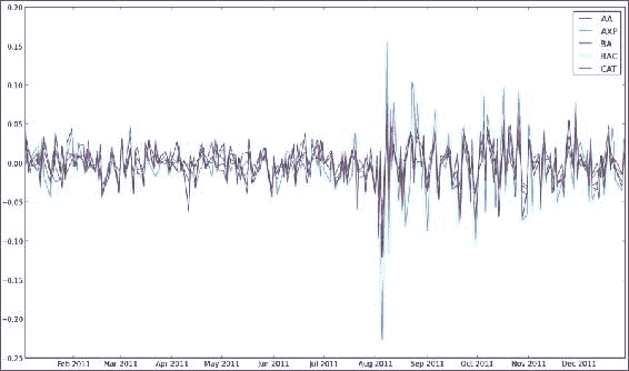
from __future__ import print_function
import pandas as pd
import matplotlib.pyplot as plt
from datetime import datetime
from matplotlib import finance
import numpy as np

# 2011 to 2012
start = datetime(2011, 01, 01)
end = datetime(2012, 01, 01)

symbols = ["AA", "AXP", "BA", "BAC", "CAT"]

quotes = [finance.quotes_historical_yahoo(symbol, start, end, asobject=True)
          for symbol in symbols]

close = np.array([q.close for q in quotes]).astype(np.float)
dates = np.array([q.date for q in quotes])

data = {}

for i, symbol in enumerate(symbols):
   data[symbol] = np.diff(np.log(close[i]))

df = pd.DataFrame(data, index=dates[0][:-1], columns=symbols)

print(df.corr())
df.plot()
plt.legend(symbols)
plt.show()

#           AA       AXP        BA       BAC       CAT
#AA   1.000000  0.768484  0.758264  0.737625  0.837643
#AXP  0.768484  1.000000  0.746898  0.760043  0.736337
#BA   0.758264  0.746898  1.000000  0.657075  0.770696
#BAC  0.737625  0.760043  0.657075  1.000000  0.657113
#CAT  0.837643  0.736337  0.770696  0.657113  1.000000

这是相关矩阵的输出：

 AA       AXP        BA       BAC       CAT
AA   1.000000  0.768484  0.758264  0.737625  0.837643
AXP  0.768484  1.000000  0.746898  0.760043  0.736337
BA   0.758264  0.746898  1.000000  0.657075  0.770696
BAC  0.737625  0.760043  0.657075  1.000000  0.657113
CAT  0.837643  0.736337  0.770696  0.657113  1.000000

显示了五只股票的对数收益图：

工作原理

我们使用了以下DataFrame方法：

函数	描述
`pandas.DataFrame()`	此函数使用指定的数据，索引（行）和列标签构造`DataFrame`。
`pandas.DataFrame.corr()`	该函数计算列的成对相关，而忽略缺失值。默认情况下，使用 Pearson 相关。
`pandas.DataFrame.plot()`	此函数使用`matplotlib`绘制数据帧。

另见

相关文档
第 4 章，“Pandas 入门书”，摘自 Ivan Idris 的书“Python 数据分析”， Packt Publishing

从 Statsmodels 中将数据作为 pandas 对象加载

statsmodels 在其发行版中有很多样本数据集。完整列表可以在这个页面中找到。

在本教程中，我们将专注于铜数据集，其中包含有关铜价，世界消费量和其他参数的信息。

准备

在开始之前，我们可能需要安装 patsy。 patsy 是描述统计模型的库。很容易看出这个库是否是必需的。只需运行代码。如果您收到与 patsy 相关的错误，请执行以下任一命令：

$ sudo easy_install patsy
$ pip install --upgrade patsy

操作步骤

在本节中，我们将从 statsmodels 中加载数据集作为 Pandas DataFrame或Series对象。

我们需要调用的函数是load_pandas()。如下加载数据：
```
data = statsmodels.api.datasets.copper.load_pandas()
```
这会将数据加载到包含 Pandas 对象的DataSet对象中。
DataSet对象具有名为exog的属性，当作为 Pandas 对象加载时，该属性将成为具有多个列的DataFrame对象。在我们的案例中，它还有一个endog属性，其中包含世界铜消费量的值。

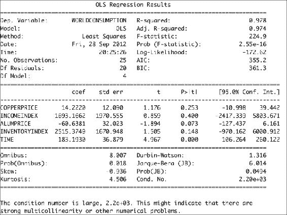
通过创建OLS对象并调用其fit()方法来执行普通的最小二乘计算，如下所示：
```
x, y = data.exog, data.endog

fit = statsmodels.api.OLS(y, x).fit()
print("Fit params", fit.params)
```
这应该打印拟合过程的结果：
```
Fit params COPPERPRICE         14.222028
INCOMEINDEX       1693.166242
ALUMPRICE          -60.638117
INVENTORYINDEX    2515.374903
TIME               183.193035
```

OLS 拟合的结果可以通过summary()方法总结如下：

print(fit.summary())

这将为我们提供以下回归结果输出：

加载铜数据集所需的代码如下：

from __future__ import print_function
import statsmodels.api

# See https://github.com/statsmodels/statsmodels/tree/master/statsmodels/datasets
data = statsmodels.api.datasets.copper.load_pandas()

x, y = data.exog, data.endog

fit = statsmodels.api.OLS(y, x).fit()
print("Fit params", fit.params)
print()
print("Summary")
print()
print(fit.summary())

工作原理

Statsmodels 的Dataset类中的数据遵循特殊格式。其中，此类具有endog和exog属性。 Statsmodels 具有load()函数，该函数将数据作为 NumPy 数组加载。相反，我们使用了load_pandas()方法，该方法将数据加载为pandas对象。我们进行了 OLS 拟合，基本上为我们提供了铜价和消费量的统计模型。

另见

相关文档

重采样时间序列数据

在此教程中，您将学习如何使用 Pandas 对时间序列进行重新采样。

操作步骤

我们将下载AAPL的每日价格时间序列数据，然后通过计算平均值将其重新采样为每月数据。我们将通过创建 Pandas DataFrame并调用其resample() 方法来做到这一点：

在创建 Pandas DataFrame之前，我们需要创建一个DatetimeIndex对象传递给DataFrame构造器。根据下载的报价数据创建索引，如下所示：
```
dt_idx = pandas.DatetimeIndex(quotes.date)
```
获得日期时间索引后，我们将其与收盘价一起使用以创建数据框：
```
df = pandas.DataFrame (quotes.close, index=dt_idx, columns=[symbol])
```

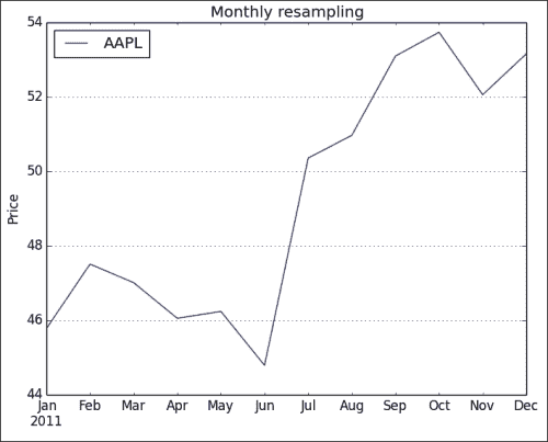
通过计算平均值，将时间序列重新采样为每月频率：

resampled = df.resample('M', how=numpy.mean)
print(resampled)

如下行所示，重新采样的时间序列每个月都有一个值：

 AAPL
2011-01-31  336.932500
2011-02-28  349.680526
2011-03-31  346.005652
2011-04-30  338.960000
2011-05-31  340.324286
2011-06-30  329.664545
2011-07-31  370.647000
2011-08-31  375.151304
2011-09-30  390.816190
2011-10-31  395.532381
2011-11-30  383.170476
2011-12-31  391.251429

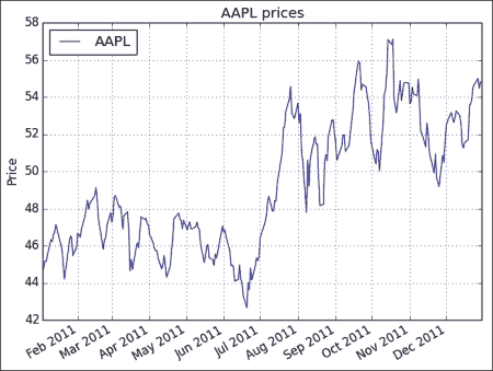
使用DataFrame plot()方法绘制数据：

df.plot()
resampled.plot()
plt.show()

原始时间序列的图如下：

重采样的数据具有较少的数据点，因此，生成的图更加混乱，如以下屏幕截图所示：

完整的重采样代码如下：

from __future__ import print_function
import pandas
import matplotlib.pyplot as plt
from datetime import datetime
from matplotlib import finance
import numpy as np

# Download AAPL data for 2011 to 2012
start = datetime(2011, 01, 01)
end = datetime(2012, 01, 01)

symbol = "AAPL"
quotes = finance.quotes_historical_yahoo(symbol, start, end, asobject=True)

# Create date time index
dt_idx = pandas.DatetimeIndex(quotes.date)

#Create data frame
df = pandas.DataFrame(quotes.close, index=dt_idx, columns=[symbol])

# Resample with monthly frequency
resampled = df.resample('M', how=np.mean)
print(resampled) 

# Plot
df.plot()
plt.title('AAPL prices')
plt.ylabel('Price')

resampled.plot()
plt.title('Monthly resampling')
plt.ylabel('Price')
plt.grid(True)
plt.show()

工作原理

我们根据日期和时间列表创建了日期时间索引。然后，该索引用于创建 Pandas DataFrame。然后，我们对时间序列数据进行了重新采样。单个字符给出重采样频率，如下所示：

每天D
每月M
每年A

resample()方法的how参数指示如何采样数据。默认为计算平均值。

另见

相关 Pandas 文档

posted @ 2023-04-12 22:49 绝不原创的飞龙阅读(77) 评论(0) 收藏举报

刷新页面返回顶部

龙哥盟

掠夺·扩张·投机·博弈

NumPy 秘籍中文第二版：6~10

六、特殊数组和通用函数

简介

创建通用函数

操作步骤

工作原理

另见

查找勾股三元组

操作步骤

工作原理

另见

使用chararray执行字符串操作

操作步骤

工作原理

另见

创建遮罩数组

操作步骤

工作原理

另见

忽略负值和极值

操作步骤

工作原理

另见

使用recarray函数创建得分表

操作步骤

工作原理

另见

七、性能分析和调试

简介

使用timeit进行性能分析

操作步骤

工作原理

另见

使用 IPython 进行分析

操作步骤

工作原理

另见

安装line_profiler

准备

操作步骤

另见

使用line_profiler分析代码

操作步骤

工作原理

另见

cProfile扩展和代码性能分析

操作步骤

另见

使用 IPython 进行调试

操作步骤

工作原理

另见

使用 PuDB 进行调试

操作步骤

另见

八、质量保证

简介

安装 Pyflakes

准备

操作步骤

另见

使用 Pyflakes 执行静态分析

操作步骤

工作原理

使用 Pylint 分析代码

准备

操作步骤

工作原理

另见

使用 Pychecker 执行静态分析

操作步骤

使用文档字符串测试代码

操作步骤

工作原理

另见

编写单元测试

注意

操作步骤

使用`chararray`执行字符串操作

使用`recarray`函数创建得分表

使用`timeit`进行性能分析

安装`line_profiler`

使用`line_profiler`分析代码

`cProfile`扩展和代码性能分析