NumPy 秘籍中文第二版：1~5

原文：NumPy Cookbook - Second Edition

协议：CC BY-NC-SA 4.0

译者：飞龙

一、使用 IPython

在本章中，我们将介绍以下秘籍：

安装 IPython
使用 IPython 作为 Shell
阅读手册页
安装 matplotlib
运行 IPython 笔记本
导出 IPython 笔记本
导入网络笔记本
配置笔记本服务器
探索 SymPy 配置文件

简介

IPython，可从 ipython.org 获得，是一个免费的开源项目，可用于 Linux，Unix，MacOSX，和 Windows。 IPython 作者仅要求您在使用 IPython 的任何科学著作中引用 IPython。 IPython 提供了用于交互式计算的架构。该项目最值得注意的部分是 IPython shell。 IPython 提供了以下组件，其中包括：

交互式 Python Shell（基于终端的 Qt 应用）
一个 Web 笔记本（在 IPython 0.12 和更高版本中可用），支持富媒体和绘图

IPython 与 Python 2.5、2.6、2.7、3.1、3.2、3.3 和 3.4 版本兼容。兼容性取决于 IPython 版本。例如，IPython 2.3.0 需要 Python 2.7 或 3.3+。

您可以在这个页面上在云中尝试 IPython 而不将其安装在系统上。与本地安装的软件相比，会有一些延迟，因此这不如真实的软件好。但是， IPython 交互式外壳程序中可用的大多数功能似乎都可用。 PythonAnywhere 也有一个 Vi(m) 编辑器，如果您喜欢 vi 的话，那显然很棒。您可以从 IPython 会话中保存和编辑文件。

安装 IPython

可以通过多种方式安装 IPython ，具体取决于您的操作系统。对于基于终端的外壳，需要依赖readline。网络笔记本需要tornado和zmq。

除了安装 IPython 外，我们还将安装setuptools，它为您提供easy_install命令。 easy_install命令是 Python 的流行package管理器。一旦拥有easy_install即可安装pip。 pip命令类似于easy_install，并添加了诸如卸载之类的选项。

操作步骤

本节介绍如何在 Windows，MacOSX 和 Linux 上安装 IPython。它还描述了如何使用easy_install和pip或从源代码安装 IPython 及其依赖项：

在 Windows 上安装 IPython 和 Setuptools：IPython 网站上提供了适用于 Python2 或 Python3 的二进制 Windows 安装程序。另见这里。

使用安装程序安装 Setuptools。然后安装pip，如下所示：
```
cd C:\Python27\scripts
python .\easy_install-27-script.py pip
```
在 MacOSX 上安装 IPython：如果需要，请安装 Apple Developer Tools（Xcode）。可以在这个页面上找到 Xcode。请遵循easy_install/pip说明或本节后面提供的从源安装的说明。
在 Linux 上安装 IPython：由于 Linux 发行版太多，因此本节将不详尽：
- 在 Debian 上，键入以下命令：
```
$ su – aptitude install ipython python-setuptools
```
- 在 Fedora 上，魔术命令如下：
```
$ su – yum install ipython python-setuptools-devel
```
- 以下命令将在 Gentoo 上安装 IPython：
```
$ su – emerge ipython
```
- 对于 Ubuntu，安装命令如下：
```
$ sudo apt-get install ipython python-setuptools
```
使用easy_install或pip安装 IPython：使用以下命令，通过easy_install安装 IPython 和本章中的秘籍所需的所有依赖项：
```
$ sudo easy_install ipython pyzmq tornado readline
```
或者，您可以通过在终端中键入以下命令，首先使用easy_install安装pip：
```
$ sudo easy_install pip
```
之后，使用pip安装 IPython：
```
$ sudo pip install ipython pyzmq tornado readline
```
从源代码安装：如果您想使用最新的开发版本，则从源代码安装适合您：
1. 从这个页面下载最新的源存档。
2. 从存档中解压缩源代码：
```
$ tar xzf ipython-<version>.tar.gz
```
3. 相反，如果您已安装 Git，则可以克隆 Git 存储库：
```
$ git clone https://github.com/ipython/ipython.git
```
4. 转到下载源中的根目录：
```
$ cd ipython
```
5. 运行安装脚本。这可能需要您使用sudo运行命令，如下所示：
```
$ sudo python setup.py install
```

工作原理

我们使用几种方法安装了 IPython。这些方法大多数都安装最新的稳定版本，但从源代码安装时除外，这将安装开发版本。

另见

来自 IPython 官方网站的说明

使用 IPython 作为 Shell

科学家和工程师习惯进行实验。 IPython 是科学家根据实验而创建的。 IPython 提供的交互式环境被许多人视为对 MATLAB，Mathematica，Maple 和 R 的直接回答。

以下是 IPython Shell 的功能列表：

制表符补全
历史机制
内联编辑
使用%run调用外部 Python 脚本的功能
调用与操作系统外壳程序交互的魔术函数的能力
访问系统命令
pylab开关
访问 Python 调试器和分析器

操作步骤

本节描述了如何使用 IPython Shell：

pylab：pylab开关会自动导入所有 SciPy，NumPy 和 matplotlib 包。没有此开关，我们将不得不自行导入这些包。

我们需要做的就是在命令行中输入以下指令：

$ ipython --pylab
Type "copyright", "credits" or "license" for more information.

IPython 2.4.1 -- An enhanced Interactive Python.
?         -> Introduction and overview of IPython's features.
%quickref -> Quick reference.
help      -> Python's own help system.
object?   -> Details about 'object', use 'object??' for extra details.

Welcome to pylab, a matplotlib-based Python environment [backend: MacOSX].
For more information, type 'help(pylab)'.

In [1]: quit()
quit() or Ctrl + D quits the IPython shell.

保存会话：我们可能希望能够返回到我们的实验。在 IPython 中，很容易保存会话以供以后使用。这是通过以下命令完成的：

In [1]: %logstart
Activating auto-logging. Current session state plus future input saved.
Filename       : ipython_log.py
Mode           : rotate
Output logging : False
Raw input log  : False
Timestamping   : False
State          : active

可以使用以下命令关闭日志记录：

In [9]: %logoff
Switching logging OFF

执行系统 Shell 命令：您可以在默认的 IPython 配置文件中通过在命令前面加上!符号来执行系统外壳命令。例如，以下输入将获取当前日期：
```
In [1]: !date
```
实际上，任何以!为前缀的行都将发送到系统外壳。我们还可以存储命令输出，如下所示：
```
In [2]: thedate = !date
In [3]: thedate
```
显示历史记录：我们可以使用%hist命令显示命令的历史记录，如下所示：
```
In [1]: a = 2 + 2

In [2]: a
Out[2]: 4

In [3]: %hist
a = 2 + 2
a
%hist
```
这是命令行界面（CLI）环境中的常见功能。我们还可以使用-g开关查询历史记录：
```
In [5]: %hist -g a = 2
 1: a = 2 + 2
```

工作原理

我们看到了许多所谓的魔术功能在起作用。这些功能以%字符开头。如果单独在行中使用魔术函数，则%前缀是可选的。

另见

IPython 作为系统外壳，来自 IPython 官方网站。

阅读手册页

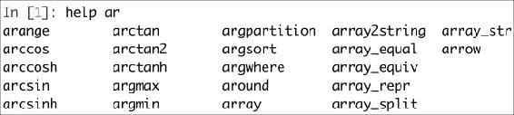
我们可以使用help命令打开有关 NumPy 函数的文档。不必知道函数的名称。我们可以输入几个字符，然后让制表符完成工作。例如，让我们浏览arange()函数的可用信息。

操作步骤

我们可以通过以下两种方式之一浏览可用信息：

调用帮助功能：调用help命令。输入该功能的几个字符，然后按Tab键（请参见以下屏幕截图）：
带问号的查询：另一个选择是在函数名称后添加问号。然后，您当然需要知道函数名称，但是不必键入help命令：
```
In [3]: arange?
```

工作原理

制表符的完成取决于readline，因此您需要确保已安装它。问号为您提供docstrings中的信息。

安装 matplotlib

matplotlib（按惯例所有小写字母）是一个非常有用的 Python 绘图库，对于以下秘籍以及以后的内容，我们将需要它。它取决于 NumPy，但很可能已经安装了 NumPy。

操作步骤

我们将看到如何在 Windows，Linux 和 MacOSX 上安装 matplotlib，以及如何从源代码安装它：

在 Windows 上安装 matplotlib：您可以使用 Enthought 发行版（也称为 Canopy）。

可能需要将msvcp71.dll文件放在您的C:\Windows\system32目录中。您可以从这里获取。
在 Linux 上安装 matplotlib：让我们看看如何在 Linux 的各种发行版中安装 matplotlib：

这是 Debian 和 Ubuntu 上的安装命令：
```
$ sudo apt-get install python-matplotlib
```
- 在 Fedora/Redhat 上的安装命令如下：
```
$ su - yum install python-matplotlib
```
从源代码安装：您可以下载 Sourceforge 的tar.gz版本或从 Git 存储库下载最新的源代码：
```
$ git clone git://github.com/matplotlib/matplotlib.git
```
下载后，请使用以下命令照常构建和安装 matplotlib：
```
$ cd matplotlib
$ sudo python setup.py install
```
在 MacOSX 上安装 matplotlib：从这里获取最新的 DMG 文件。您还可以使用 Mac Ports，Fink 或 Homebrew 包管理器。

另见

matplotlib 官方文档中的说明
在这里中说明了如何在 SciPy 栈中安装。

运行 IPython 笔记本

IPython 具有一项令人兴奋的功能-网络笔记本。所谓的笔记本服务器可以通过 Web 服务笔记本电脑。现在，我们可以启动笔记本服务器并获得基于 Web 的 IPython 环境。该环境具有常规 IPython 环境具有的大多数功能。 IPython 笔记本的功能包括：

显示图像和内嵌图
在文本单元格中使用 HTML 和 Markdown（这是一种简化的类似 HTML 的语言，请参见这里）
笔记本的导入导出

准备

在开始之前，我们应确保已安装所有必需的软件。依赖于tornado和zmq。有关更多信息，请参见本章中的“安装 IPython”秘籍。

操作步骤

运行笔记本：我们可以使用以下命令启动笔记本：
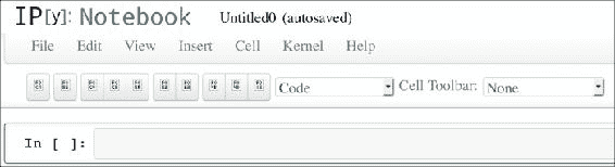
```
$ ipython notebook

[NotebookApp] Using existing profile dir: u'/Users/ivanidris/.ipython/profile_default'
[NotebookApp] The IPython Notebook is running at: http://127.0.0.1:8888
[NotebookApp] Use Control-C to stop this server and shut down all kernels.
```
如您所见，我们正在使用默认配置文件。服务器在本地计算机上的端口 8888 上启动。稍后，您将在本章中学习如何配置这些设置。笔记本在默认浏览器中打开；这也是可配置的（请参见以下屏幕截图）：

IPython 在启动笔记本的目录中列出了所有笔记本。在本示例中，未找到笔记本。可以通过按Ctrl + C停止服务器。
以pylab模式运行笔记本：使用以下命令以pylab模式运行网络笔记本：
```
$ ipython notebook --pylab
```
这将加载SciPy，NumPy和matplotlib模块。
运行带有嵌入式图形的笔记本：我们可以使用以下命令，通过inline指令显示嵌入式 matplotlib 图：
```
$ ipython notebook --pylab inline
```
以下步骤演示了 IPython 笔记本的功能：
1. 单击新笔记本按钮以创建新笔记本。
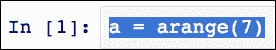
2. 使用arange()函数创建一个数组。输入以下屏幕快照中所示的命令，然后单击单元格 / 运行：
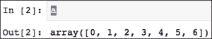
3. 接下来输入以下命令，然后按Enter。您将在Out [2]中看到输出，如以下屏幕截图所示：
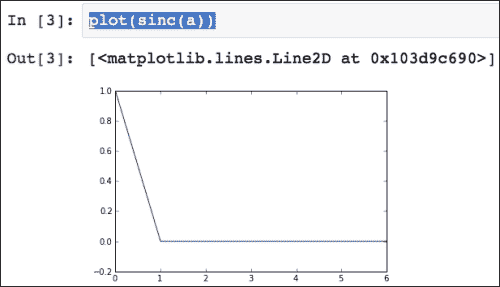
4. 将 sinc()函数应用于数组并绘制结果，如以下屏幕快照所示：

工作原理

内联选项使可以显示内联 matplotlib 图。与pylab模式结合使用时，无需导入 NumPy，SciPy 和 matplotlib 包。

另见

本章中的“安装 IPython”秘籍
笔记本的示例
sinc()函数的文档
plot()函数的文档

导出 IPython 笔记本

有时，您想与朋友或同事交换笔记本。网络笔记本提供了几种导出数据的方法。

操作步骤

可以使用以下选项导出 Web 笔记本：

打印选项：打印按钮实际上并未打印笔记本，但允许您将笔记本导出为 PDF 或 HTML 文档。

下载笔记本：使用“下载”按钮将笔记本下载到您选择的位置。我们可以指定将笔记本下载为.py文件（只是普通的 Python 程序），还是下载为 JSON 格式的.ipynb文件。导出后，我们在前一个秘籍中创建的笔记本如下所示：

{
 "metadata": {
  "name": "Untitled1"
 }, 
 "nbformat": 2, 
 "worksheets": [
  {
    "cells": [
    {
      "cell_type": "code", 
      "collapsed": false, 
      "input": [
        "plot(sinc(a))"
      ], 
      "language": "python", 
      "outputs": [
      {
        "output_type": "pyout", 
        "prompt_number": 3, 
        "text": [
          "[<matplotlib.lines.Line2D at 0x103d9c690>]"
        ]
      }, 
      {
        "output_type": "display_data", 
        "png": "iVBORw0KGgoAAAANSUhEUgAAAXkAAAD9CAYAAABZVQdHAAAABHNCSVQICAgIf...
          mgkAAAAASUVORK5CYII=\n"
      }
      ], 
      "prompt_number": 3
    }
    ]
  }
  ]
}

注意

为简洁起见，一些文本已被省略。该文件不适合编辑甚至阅读，但如果忽略图像表示部分，则可读性很强。有关 JSON 的更多信息，请参见这里。

保存笔记本：使用保存按钮保存笔记本。这会自动以本地 JSON 格式.ipynb导出笔记本。该文件将存储在最初启动 IPython 的目录中。

导入网络笔记本

可以将 Python 脚本作为 Web 笔记本导入。显然，我们也可以导入以前导出的笔记本。

操作步骤

此秘籍向您展示如何将 Python 脚本作为 Web 笔记本导入。

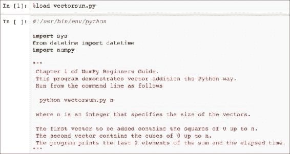
使用以下命令加载 Python 脚本：

% load vectorsum.py

以下屏幕截图显示了从“NumPy 入门指南”加载vectorsum.py后进入笔记本页面的示例：

配置笔记本服务器

公共笔记本服务器需要安全。您应该设置一个密码并使用 SSL 证书来连接它。我们需要证书来通过 HTTPS 提供安全的通信（有关更多信息，请参见这里）。 HTTPS 在互联网上广泛使用的标准 HTTP 协议之上添加了一个安全层。 HTTPS 还对从客户端发送到服务器并返回的数据进行加密。证书颁发机构通常是为网站颁发证书的商业组织。 Web 浏览器具有证书颁发机构的知识，并且可以识别证书。网站管理员需要创建证书并由证书颁发机构签名。

操作步骤

以下步骤描述了如何配置安全的笔记本服务器：

我们可以从 IPython 生成密码。启动一个新的 IPython 会话并输入以下命令：
```
In [1]: from IPython.lib import passwd

In [2]: passwd()
Enter password: 
Verify password:
Out[2]: 'sha1:0e422dfccef2:84cfbcbb3ef95872fb8e23be3999c123f862d856'
```
在第二个输入行，将提示您输入密码。您需要记住该密码。生成一个长字符串。复制此字符串，因为稍后将需要它。

要创建 SSL 证书，您需要在路径中使用openssl命令。

设置openssl命令不是火箭科学，但这可能很棘手。不幸的是，这超出了本书的范围。好的一面是，在线上有很多教程可以帮助您进一步发展。

执行以下命令，以mycert.pem为名称创建证书：

$ openssl req -x509 -nodes -days 365 -newkey rsa:1024 -keyout mycert.pem -out mycert.pem
Generating a 1024 bit RSA private key
......++++++
........................++++++
writing new private key to 'mycert.pem'
-----
You are about to be asked to enter information that will be incorporated
into your certificate request.
What you are about to enter is what is called a Distinguished Name or a DN.
There are quite a few fields but you can leave some blank
For some fields there will be a default value,
If you enter '.', the field will be left blank.
-----
Country Name (2 letter code) [AU]:
State or Province Name (full name) [Some-State]:
Locality Name (eg, city) []:
Organization Name (eg, company) [Internet Widgits Pty Ltd]:
Organizational Unit Name (eg, section) []:
Common Name (eg, YOUR name) []:
Email Address []:

openssl工具提示您填写一些字段。有关更多信息，请查看相关的手册页（手册页的缩写），如下所示：

$ man openssl

使用以下命令为服务器创建特殊的配置文件：
```
$ ipython profile create nbserver
```
编辑配置文件。在此示例中，可以在~/.ipython/profile_nbserver/ipython_notebook_config.py中找到。

配置文件很大，因此我们将省略其中的大多数行。我们至少需要更改的行如下：
```
c.NotebookApp.certfile = u'/absolute/path/to/your/certificate'
c.NotebookApp.password = u'sha1:b...your password'
c.NotebookApp.port = 9999
```
请注意，我们指向的是我们创建的 SSL 证书。我们设置了密码，并将端口更改为 9999。

使用以下命令，启动服务器以检查更改是否有效：

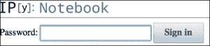
$ ipython notebook --profile=nbserver
[NotebookApp] Using existing profile dir: u'/Users/ivanidris/.ipython/profile_nbserver'
[NotebookApp] The IPython Notebook is running at: https://127.0.0.1:9999
[NotebookApp] Use Control-C to stop this server and shut down all kernels.

服务器在端口 9999 上运行，您需要通过 HTTPS 连接到它。如果一切顺利，您应该会看到一个登录页面。另外，您可能需要在浏览器中接受安全例外。

工作原理

我们为公共服务器创建了一个特殊的配置文件。已经有一些样本概要文件，例如默认概要文件。创建配置文件后，将使用配置文件将profile_<profilename>文件夹添加到.ipython目录。然后可以使用--profile=<profile_name>命令行选项加载配置文件。我们可以使用以下命令列出配置文件：

$ ipython profile list

Available profiles in IPython:
 cluster
 math
 pysh
 python3

 The first request for a bundled profile will copy it
 into your IPython directory (/Users/ivanidris/.ipython),
 where you can customize it.

Available profiles in /Users/ivanidris/.ipython:
 default
 nbserver
 sh

另见

探索 SymPy 配置文件

IPython 有一个示例 SymPy 配置文件。 SymPy 是一个 Python 符号数学库。我们可以简化代数表达式或区分函数，类似于 Mathematica 和 Maple。显然，SymPy 是一款有趣的软件，但对于我们穿越 NumPy 的过程而言并不是必需的。将此视为可选或额外的秘籍。就像甜点一样，可以随意跳过它，尽管您可能会错过本章中最甜的部分。

准备

使用easy_install或pip安装 SymPy：

$ sudo easy_install sympy
$ sudo pip install sympy

操作步骤

以下步骤将帮助您探索 SymPy 配置文件：

查看配置文件，该文件位于~/.ipython/profile_sympy/ipython_config.py。内容如下：

c = get_config()
app = c.InteractiveShellApp

# This can be used at any point in a config file to load a sub config
# and merge it into the current one.
load_subconfig('ipython_config.py', profile='default')

lines = """
from __future__ import division
from sympy import *
x, y, z, t = symbols('x y z t')
k, m, n = symbols('k m n', integer=True)
f, g, h = symbols('f g h', cls=Function)
"""

# You have to make sure that attributes that are containers already
# exist before using them.  Simple assigning a new list will override
# all previous values.

if hasattr(app, 'exec_lines'):
 app.exec_lines.append(lines)
else:
 app.exec_lines = [lines]

# Load the sympy_printing extension to enable nice printing of sympy expr's.
if hasattr(app, 'extensions'):
 app.extensions.append('sympyprinting')
else:
 app.extensions = ['sympyprinting']

此代码完成以下任务：

加载默认配置文件
导入 SymPy 包
定义符号

使用以下命令以 SymPy 配置文件启动 IPython：
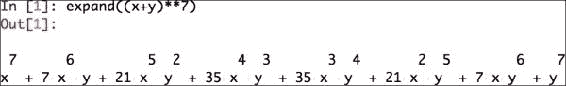
```
$ ipython --profile=sympy
```
使用以下屏幕快照中所示的命令扩展代数表达式：

另见

SymPy 主页

二、高级索引和数组概念

在本章中，我们将介绍以下秘籍：

安装 SciPy
安装 PIL
调整图像大小
比较视图和副本
翻转 Lena
花式索引
位置列表索引
布尔值索引
数独的步幅技巧
广播数组

简介

NumPy 以其高效的数组而闻名。之所以成名，部分原因是索引容易。我们将演示使用图像的高级索引技巧。在深入研究索引之前，我们将安装必要的软件 -- SciPy 和 PIL。如果您认为有此需要，请参阅第 1 章“使用 IPython”的“安装 matplotlib”秘籍。

在本章和其他章中，我们将使用以下导入：

import numpy as np 
import matplotlib.pyplot as plt
import scipy

我们还将尽可能为print() Python 函数使用最新的语法。

注意

Python2 是仍然很流行的主要 Python 版本，但与 Python3 不兼容。Python2 直到 2020 年才正式失去支持。主要区别之一是print()函数的语法。本书使用的代码尽可能与 Python2 和 Python3 兼容。

本章中的一些示例涉及图像处理。为此，我们将需要 Python 图像库（PIL），但不要担心；必要时会在本章中提供帮助您安装 PIL 和其他必要 Python 软件的说明和指示。

安装 SciPy

SciPy 是科学的 Python 库，与 NumPy 密切相关。实际上，SciPy 和 NumPy 在很多年前曾经是同一项目。就像 NumPy 一样，SciPy 是一个开放源代码项目，已获得 BSD 许可。在此秘籍中，我们将安装 SciPy。 SciPy 提供高级功能，包括统计，信号处理，线性代数，优化，FFT，ODE 求解器，插值，特殊功能和积分。 NumPy 有一些重叠，但是 NumPy 主要提供数组功能。

准备

在第 1 章，“使用 IPython”中，我们讨论了如何安装setuptools和pip。如有必要，请重新阅读秘籍。

操作步骤

在此秘籍中，我们将完成安装 SciPy 的步骤：

从源安装：如果已安装 Git，则可以使用以下命令克隆 SciPy 存储库：
```
$ git clone https://github.com/scipy/scipy.git

$ python setup.py build
$ python setup.py install --user
```
这会将 SciPy 安装到您的主目录。它需要 Python 2.6 或更高版本。

在构建之前，您还需要安装 SciPy 依赖的以下包：
- BLAS和LAPACK库
- C 和 Fortran 编译器
您可能已经在 NumPy 安装过程中安装了此软件。
在 Linux 上安装 SciPy：大多数 Linux 发行版都包含 SciPy 包。我们将遵循一些流行的 Linux 发行版中的必要步骤（您可能需要以 root 用户身份登录或具有sudo权限）：
- 为了在 RedHat，Fedora 和 CentOS 上安装 SciPy，请从命令行运行以下指令：
```
$ yum install python-scipy
```
- 为了在 Mandriva 上安装 SciPy，请运行以下命令行指令：
```
$ urpmi python-scipy
```
- 为了在 Gentoo 上安装 SciPy，请运行以下命令行指令：
```
$ sudo emerge scipy
```
- 在 Debian 或 Ubuntu 上，我们需要输入以下指令：
```
$ sudo apt-get install python-scipy
```
在 MacOSX 上安装 SciPy：需要 Apple Developer Tools（XCode），因为它包含BLAS和LAPACK库。可以在 App Store 或 Mac 随附的安装 DVD 中找到它。或者您可以从 Apple Developer 的连接网站获取最新版本。确保已安装所有内容，包括所有可选包。

您可能已经为 NumPy 安装了 Fortran 编译器。 gfortran的二进制文件可以在这个链接中找到。
使用easy_install或pip安装 SciPy：您可以使用以下两个命令中的任何一个来安装 SciPy（sudo的需要取决于权限）：
```
$ [sudo] pip install scipy
$ [sudo] easy_install scipy

```** 
```
在 Windows 上安装：如果已经安装 Python，则首选方法是下载并使用二进制发行版。或者，您可以安装 Anaconda 或 Enthought Python 发行版，该发行版与其他科学 Python 包一起提供。
检查安装：使用以下代码检查 SciPy 安装：
```
import scipy
print(scipy.__version__)
print(scipy.__file__)
```
这应该打印正确的 SciPy 版本。

工作原理

大多数包管理器都会为您解决依赖项（如果有）。但是，在某些情况下，您需要手动安装它们。这超出了本书的范围。

另见

如果遇到问题，可以在以下位置寻求帮助：

freenode的#scipy IRC 频道
SciPy 邮件列表

安装 PIL

PIL（Python 图像库）是本章中进行图像处理的先决条件。如果愿意，可以安装 Pillow，它是 PIL 的分支。有些人喜欢 Pillow API；但是，我们不会在本书中介绍其安装。

操作步骤

让我们看看如何安装 PIL：

在 Windows 上安装 PIL：使用 Windows 中的 PIL 可执行文件安装 PIL。
在 Debian 或 Ubuntu 上安装：在 Debian 或 Ubuntu 上，使用以下命令安装 PIL：
```
$ sudo apt-get install python-imaging
```
使用easy_install或pip安装：在编写本书时，似乎 RedHat，Fedora 和 CentOS 的包管理器没有对 PIL 的直接支持。因此，如果您使用的是这些 Linux 发行版之一，请执行此步骤。

使用以下任一命令安装：
```
$ easy_install PIL
$ sudo pip install PIL
```

另见

可在这里找到有关 PILLOW（PIL 的分支）的说明。

调整图像大小

在此秘籍中，我们将把 Lena 的样例图像（在 SciPy 发行版中可用）加载到数组中。顺便说一下，本章不是关于图像操作的。我们将只使用图像数据作为输入。

注意

Lena Soderberg 出现在 1972 年的《花花公子》杂志中。由于历史原因，这些图像之一经常用于图像处理领域。不用担心，该图像完全可以安全工作。

我们将使用repeat()函数调整图像大小。此函数重复一个数组，这意味着在我们的用例中按一定的大小调整图像大小。

准备

此秘籍的前提条件是必须安装 SciPy，matplotlib 和 PIL。看看本章和第 1 章，“使用 IPython”的相应秘籍。

操作步骤

通过以下步骤调整图像大小：

首先，导入SciPy。 SciPy 具有lena()函数。它用于将图像加载到 NumPy 数组中：
```
lena = scipy.misc.lena()
```
从 0.10 版本开始发生了一些重构，因此，如果您使用的是旧版本，则正确的代码如下：
```
lena = scipy.lena()
```
使用numpy.testing包中的assert_equal()函数检查 Lena 数组的形状-这是可选的完整性检查测试：
```
np.testing.assert_equal((LENA_X, LENA_Y), lena.shape)
```
使用repeat()函数调整 Lena 数组的大小。我们在x和y方向上给此函数一个调整大小的因子：
```
resized = lena.repeat(yfactor, axis=0).repeat(xfactor, axis=1)
```

我们将在同一网格的两个子图中绘制 Lena 图像和调整大小后的图像。使用以下代码在子图中绘制 Lena 数组：

plt.subplot(211)
plt.title("Lena")
plt.axis("off")
plt.imshow(lena)

matplotlib subplot()函数创建一个子图。此函数接受一个三位整数作为参数，其中第一位是行数，第二位是列数，最后一位是子图的索引，从 1 开始。imshow()函数显示图像。最后，show()函数显示最终结果。

将调整大小后的数组绘制在另一个子图中并显示它。索引现在为 2：

plt.subplot(212)
plt.title("Resized")
plt.axis("off")
plt.imshow(resized)
plt.show()

以下屏幕截图显示了结果，以及原始图像（第一幅）和调整大小后的图像（第二幅）：

以下是本书代码包中resize_lena.py文件中该秘籍的完整代码：

import scipy.misc
import matplotlib.pyplot as plt
import numpy as np

# This script resizes the Lena image from Scipy.

# Loads the Lena image into an array
lena = scipy.misc.lena()

#Lena's dimensions
LENA_X = 512
LENA_Y = 512

#Check the shape of the Lena array
np.testing.assert_equal((LENA_X, LENA_Y), lena.shape)

# Set the resize factors
yfactor = 2
xfactor = 3

# Resize the Lena array
resized = lena.repeat(yfactor, axis=0).repeat(xfactor, axis=1)

#Check the shape of the resized array
np.testing.assert_equal((yfactor * LENA_Y, xfactor * LENA_Y), resized.shape)

# Plot the Lena array
plt.subplot(211)
plt.title("Lena")
plt.axis("off")
plt.imshow(lena)

#Plot the resized array
plt.subplot(212)
plt.title("Resized")
plt.axis("off")
plt.imshow(resized)
plt.show()

工作原理

repeat()函数重复数组，在这种情况下，这会导致原始图像的大小改变。 subplot() matplotlib 函数创建一个子图。 imshow()函数显示图像。最后，show()函数显示最终结果。

另见

第 1 章“使用 IPython”中的“安装 matplotlib”
本章中的“安装 SciPy”
本章中的“安装 PIL”
这个页面中介绍了repeat()函数。

创建视图和副本

了解何时处理共享数组视图以及何时具有数组数据的副本，这一点很重要。例如，切片将创建一个视图。这意味着，如果您将切片分配给变量，然后更改基础数组，则此变量的值将更改。我们将根据著名的 Lena 图像创建一个数组，复制该数组，创建一个视图，最后修改视图。

准备

前提条件与先前的秘籍相同。

操作步骤

让我们创建 Lena 数组的副本和视图：

创建 Lena 数组的副本：
```
acopy = lena.copy()
```
创建数组的视图：
```
aview = lena.view()
```

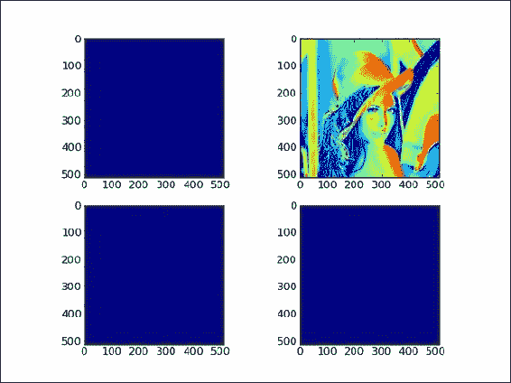
使用flat迭代器将视图的所有值设置为0：

aview.flat = 0

最终结果是只有一个图像（与副本相关的图像）显示了花花公子模型。其他图像完全消失：

以下是本教程的代码，显示了本书代码包中copy_view.py文件中数组视图和副本的行为：

import scipy.misc
import matplotlib.pyplot as plt

lena = scipy.misc.lena()
acopy = lena.copy()
aview = lena.view()

# Plot the Lena array
plt.subplot(221)
plt.imshow(lena)

#Plot the copy
plt.subplot(222)
plt.imshow(acopy)

#Plot the view
plt.subplot(223)
plt.imshow(aview)

# Plot the view after changes
aview.flat = 0
plt.subplot(224)
plt.imshow(aview)

plt.show()

工作原理

如您所见，通过在程序结尾处更改视图，我们更改了原始 Lena 数组。这样就产生了三张蓝色（如果您正在查看黑白图像，则为空白）图像-复制的数组不受影响。重要的是要记住，视图不是只读的。

另见

NumPy view()函数的文档位于这里

翻转 Lena

我们将翻转 SciPy Lena 图像-当然，所有这些都是以科学的名义，或者至少是作为演示。除了翻转图像，我们还将对其进行切片并对其应用遮罩。

操作步骤

步骤如下：

使用以下代码围绕垂直轴翻转 Lena 数组：
```
plt.imshow(lena[:,::-1])
```
从图像中切出一部分并将其绘制出来。在这一步中，我们将看一下 Lena 数组的形状。该形状是表示数组大小的元组。以下代码有效地选择了花花公子图片的左上象限：
```
plt.imshow(lena[:lena.shape[0]/2,:lena.shape[1]/2])
```

通过在 Lena 数组中找到所有偶数的值，对图像应用遮罩（这对于演示目的来说是任意的）。复制数组并将偶数值更改为 0。这样会在图像上放置很多蓝点（如果您正在查看黑白图像，则会出现暗点）：

mask = lena % 2 == 0
masked_lena = lena.copy()
masked_lena[mask] = 0

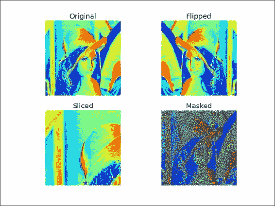
所有这些工作都会产生2 x 2的图像网格，如以下屏幕截图所示：

这是本书代码包中flip_lena.py文件中此秘籍的完整代码：

import scipy.misc
import matplotlib.pyplot as plt

# Load the Lena array
lena = scipy.misc.lena()

# Plot the Lena array
plt.subplot(221)
plt.title('Original')
plt.axis('off')
plt.imshow(lena)

#Plot the flipped array
plt.subplot(222)
plt.title('Flipped')
plt.axis('off')
plt.imshow(lena[:,::-1])

#Plot a slice array
plt.subplot(223)
plt.title('Sliced')
plt.axis('off')
plt.imshow(lena[:lena.shape[0]/2,:lena.shape[1]/2])

# Apply a mask
mask = lena % 2 == 0
masked_lena = lena.copy()
masked_lena[mask] = 0
plt.subplot(224)
plt.title('Masked')
plt.axis('off')
plt.imshow(masked_lena)

plt.show()

另见

第 1 章“使用 IPython”中的“安装 matplotlib”
本章中的“安装 SciPy”
本章中的“安装 PIL”

花式索引

在本教程中，我们将应用花式索引将 Lena 图像的对角线值设置为 0。这将沿着对角线绘制黑线并交叉，这不是因为图像有问题，而仅仅作为练习。花式索引是不涉及整数或切片的索引；这是正常的索引编制。

操作步骤

我们将从第一个对角线开始：

将第一个对角线的值设置为0。

要将对角线值设置为0，我们需要为x和y值定义两个不同的范围：
```
lena[range(xmax), range(ymax)] = 0
```

将另一个对角线的值设置为0。

要设置另一个对角线的值，我们需要一组不同的范围，但是原理保持不变：

lena[range(xmax-1,-1,-1), range(ymax)] = 0

最后，我们得到带有对角线标记的图像，如以下屏幕截图所示：

以下是本书代码集中fancy.py文件中该秘籍的完整代码：

import scipy.misc
import matplotlib.pyplot as plt

# This script demonstrates fancy indexing by setting values
# on the diagonals to 0.

# Load the Lena array
lena = scipy.misc.lena()
xmax = lena.shape[0]
ymax = lena.shape[1]

# Fancy indexing
# Set values on diagonal to 0
# x 0-xmax
# y 0-ymax
lena[range(xmax), range(ymax)] = 0

# Set values on other diagonal to 0
# x xmax-0
# y 0-ymax
lena[range(xmax-1,-1,-1), range(ymax)] = 0

# Plot Lena with diagonal lines set to 0
plt.imshow(lena)
plt.show()

工作原理

我们为x值和y值定义了单独的范围。这些范围用于索引 Lena 数组。花式索引是基于内部 NumPy 迭代器对象执行的。执行以下步骤：

创建迭代器对象。
迭代器对象绑定到数组。
数组元素通过迭代器访问。

另见

花式索引的实现文档

位置列表索引

让我们使用ix_()函数来随机播放 Lena 图像。此函数根据多个序列创建网格。

操作步骤

我们将从随机改组数组索引开始：

使用numpy.random模块的shuffle()函数创建随机索引数组：

def shuffle_indices(size):
   arr = np.arange(size)
   np.random.shuffle(arr)

   return arr

绘制乱序的索引：

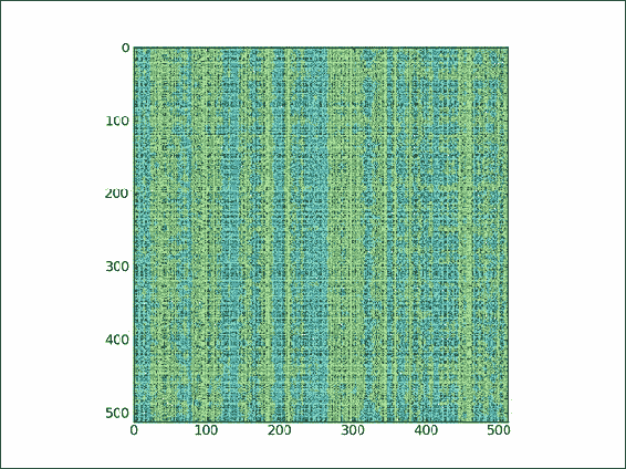
plt.imshow(lena[np.ix_(xindices, yindices)])

我们得到的是一张完全打乱的 Lena 图像，如以下屏幕截图所示：

这是本书代码包中ix.py文件中秘籍的完整代码：

import scipy.misc
import matplotlib.pyplot as plt
import numpy as np

# Load the Lena array
lena = scipy.misc.lena()
xmax = lena.shape[0]
ymax = lena.shape[1]

def shuffle_indices(size):
   '''
   Shuffles an array with values 0 - size
   '''
   arr = np.arange(size)
   np.random.shuffle(arr)

   return arr

xindices = shuffle_indices(xmax)
np.testing.assert_equal(len(xindices), xmax)
yindices = shuffle_indices(ymax)
np.testing.assert_equal(len(yindices), ymax)

# Plot Lena
plt.imshow(lena[np.ix_(xindices, yindices)])
plt.show()

另见

ix_()函数的文档页面

布尔值索引

布尔索引是基于布尔数组的索引，属于奇特索引的类别。

操作步骤

我们将这种索引技术应用于图像：

在对角线上带有点的图像。

这在某种程度上类似于本章中的“花式索引”秘籍。这次，我们在图像的对角线上选择模4：

def get_indices(size):
   arr = np.arange(size)
   return arr % 4 == 0

然后，我们只需应用此选择并绘制点：

lena1 = lena.copy() 
xindices = get_indices(lena.shape[0])
yindices = get_indices(lena.shape[1])
lena1[xindices, yindices] = 0
plt.subplot(211)
plt.imshow(lena1)

在最大值的四分之一到四分之三之间选择数组值，并将它们设置为0：

lena2[(lena > lena.max()/4) & (lena < 3 * lena.max()/4)] = 0

带有两个新图像的图看起来类似于以下屏幕截图所示：

这是本书代码包中boolean_indexing.py文件中该秘籍的完整代码：

import scipy.misc
import matplotlib.pyplot as plt
import numpy as np

# Load the Lena array
lena = scipy.misc.lena()

def get_indices(size):
   arr = np.arange(size)
   return arr % 4 == 0

# Plot Lena
lena1 = lena.copy() 
xindices = get_indices(lena.shape[0])
yindices = get_indices(lena.shape[1])
lena1[xindices, yindices] = 0
plt.subplot(211)
plt.imshow(lena1)

lena2 = lena.copy() 
# Between quarter and 3 quarters of the max value
lena2[(lena > lena.max()/4) & (lena < 3 * lena.max()/4)] = 0
plt.subplot(212)
plt.imshow(lena2)

plt.show()

工作原理

由于布尔值索引是一种花式索引，因此它的工作方式基本相同。这意味着索引是在特殊的迭代器对象的帮助下发生的。

另见

“花式索引”

数独的步幅技巧

ndarray 类具有strides字段，它是一个元组，指示通过数组时要在每个维中步进的字节数。让我们对将数独谜题拆分为3 x 3正方形的问题应用一些大步技巧。

注意

对数独的规则进行解释超出了本书的范围。简而言之，数独谜题由3 x 3的正方形组成。这些正方形均包含九个数字。有关更多信息，请参见这里。

操作步骤

应用如下的跨步技巧：

让我们定义sudoku数组。此数组充满了一个实际的已解决的数独难题的内容：

sudoku = np.array([
    [2, 8, 7, 1, 6, 5, 9, 4, 3],
    [9, 5, 4, 7, 3, 2, 1, 6, 8],
    [6, 1, 3, 8, 4, 9, 7, 5, 2],
    [8, 7, 9, 6, 5, 1, 2, 3, 4],
    [4, 2, 1, 3, 9, 8, 6, 7, 5],
    [3, 6, 5, 4, 2, 7, 8, 9, 1],
    [1, 9, 8, 5, 7, 3, 4, 2, 6],
    [5, 4, 2, 9, 1, 6, 3, 8, 7],
    [7, 3, 6, 2, 8, 4, 5, 1, 9]
    ])

ndarray的itemsize字段为我们提供了数组中的字节数。给定itemsize，请计算步幅：
```
strides = sudoku.itemsize * np.array([27, 3, 9, 1])
```

现在我们可以使用np.lib.stride_tricks模块的as_strided()函数将拼图分解成正方形：

squares = np.lib.stride_tricks.as_strided(sudoku, shape=shape, strides=strides)
print(squares)

该代码打印单独的数独正方形，如下所示：

[[[[2 8 7]
    [9 5 4]
    [6 1 3]]

  [[1 6 5]
    [7 3 2]
    [8 4 9]]

  [[9 4 3]
    [1 6 8]
    [7 5 2]]]

 [[[8 7 9]
    [4 2 1]
    [3 6 5]]

  [[6 5 1]
    [3 9 8]
    [4 2 7]]

  [[2 3 4]
    [6 7 5]
    [8 9 1]]]

 [[[1 9 8]
    [5 4 2]
    [7 3 6]]

  [[5 7 3]
    [9 1 6]
    [2 8 4]]

  [[4 2 6]
    [3 8 7]
    [5 1 9]]]]

以下是本书代码包中strides.py文件中此秘籍的完整源代码：

import numpy as np

sudoku = np.array([
   [2, 8, 7, 1, 6, 5, 9, 4, 3],
   [9, 5, 4, 7, 3, 2, 1, 6, 8],
   [6, 1, 3, 8, 4, 9, 7, 5, 2],
   [8, 7, 9, 6, 5, 1, 2, 3, 4],
   [4, 2, 1, 3, 9, 8, 6, 7, 5],
   [3, 6, 5, 4, 2, 7, 8, 9, 1],
   [1, 9, 8, 5, 7, 3, 4, 2, 6],
   [5, 4, 2, 9, 1, 6, 3, 8, 7],
   [7, 3, 6, 2, 8, 4, 5, 1, 9]
   ])

shape = (3, 3, 3, 3)

strides = sudoku.itemsize * np.array([27, 3, 9, 1])

squares = np.lib.stride_tricks.as_strided(sudoku, shape=shape, strides=strides)
print(squares)

工作原理

我们应用了跨步技巧，将数独谜题拆分为3 x 3的正方形。步幅告诉我们通过数独数组时每一步需要跳过的字节数。

另见

strides属性的文档在这里

广播数组

在不知道的情况下，您可能已经广播了数组。简而言之，即使操作数的形状不同，NumPy 也会尝试执行操作。在此秘籍中，我们将一个数组和一个标量相乘。标量被扩展为数组操作数的形状，然后执行乘法。我们将下载一个音频文件并制作一个更安静的新版本。

操作步骤

让我们从读取 WAV 文件开始：

我们将使用标准的 Python 代码下载 Austin Powers 的音频文件。 SciPy 具有 WAV 文件模块，可让您加载声音数据或生成 WAV 文件。如果已安装 SciPy，则我们应该已经有此模块。 read()函数返回data数组和采样率。在此示例中，我们仅关心数据：
```
sample_rate, data = scipy.io.wavfile.read(WAV_FILE)
```
使用 matplotlib 绘制原始 WAV 数据。将子图命名为Original：
```
plt.subplot(2, 1, 1)
plt.title("Original")
plt.plot(data)
```
现在，我们将使用 NumPy 制作更安静的音频样本。这只是通过与常量相乘来创建具有较小值的新数组的问题。这就是广播魔术发生的地方。最后，由于 WAV 格式，我们需要确保与原始数组具有相同的数据类型：
```
newdata = data * 0.2
newdata = newdata.astype(np.uint8)
```

可以将新数组写入新的 WAV 文件，如下所示：

scipy.io.wavfile.write("quiet.wav",
    sample_rate, newdata)

使用 matplotlib 绘制新数据数组：

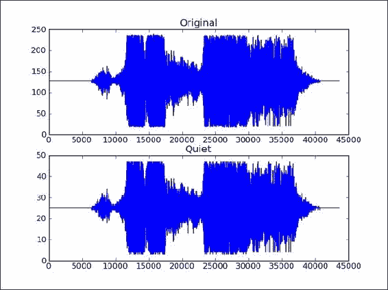
plt.subplot(2, 1, 2)
plt.title("Quiet")
plt.plot(newdata)

plt.show()

结果是原始 WAV 文件数据和具有较小值的新数组的图，如以下屏幕快照所示：

这是本书代码包中broadcasting.py文件中该秘籍的完整代码：

import scipy.io.wavfile
import matplotlib.pyplot as plt
import urllib2
import numpy as np

# Download audio file
response = urllib2.urlopen('http://www.thesoundarchive.com/austinpowers/smashingbaby.wav')
print(response.info())
WAV_FILE = 'smashingbaby.wav'
filehandle = open(WAV_FILE, 'w')
filehandle.write(response.read())
filehandle.close()
sample_rate, data = scipy.io.wavfile.read(WAV_FILE)
print("Data type", data.dtype, "Shape", data.shape)

# Plot values original audio
plt.subplot(2, 1, 1)
plt.title("Original")
plt.plot(data)

# Create quieter audio
newdata = data * 0.2
newdata = newdata.astype(np.uint8)
print("Data type", newdata.dtype, "Shape", newdata.shape)

# Save quieter audio file
scipy.io.wavfile.write("quiet.wav",
    sample_rate, newdata)

# Plot values quieter file
plt.subplot(2, 1, 2)
plt.title("Quiet")
plt.plot(newdata)

plt.show()

另见

以下链接提供了更多背景信息：

三、掌握常用函数

在本章中，我们将介绍许多常用函数：

sqrt()，log()，arange()，astype()和sum()
ceil()，modf()，where()，ravel()和take()
sort()和outer()
diff()，sign()和eig()
histogram()和polyfit()
compress()和randint()

我们将在以下秘籍中讨论这些功能：

斐波纳契数求和
查找素因数
查找回文数
稳态向量
发现幂律
逢低定期交易
随机模拟交易
用 Eratosthenes 筛子来筛选质数

简介

本章介绍常用的 NumPy 函数。这些是您每天将要使用的函数。显然，用法可能与您不同。 NumPy 函数太多，以至于几乎不可能全部了解，但是本章中的函数是我们应该熟悉的最低要求。

斐波纳契数求和

在此秘籍中，我们将求和值不超过 400 万的斐波纳契数列中的偶数项。斐波那契数列是从零开始的整数序列，其中每个数字都是前两个数字的和，但（当然）前两个数字除外，零和一（0、1、1、2、3、5、8、13、21、34、55、89 ...）。

该序列由斐波那契（Fibonacci）在 1202 年发布，最初不包含零。实际上，早在几个世纪以前，印度数学家就已经知道了它。斐波那契数在数学，计算机科学和生物学中都有应用。

注意

有关更多信息，请阅读 Wikipedia 关于斐波那契数字的文章。

该秘籍使用基于黄金比例的公式，这是一个无理数，具有与pi相当的特殊性质。黄金比例由以下公式给出：

我们将使用sqrt()，log()，arange()，astype()和sum()函数。斐波那契数列的递归关系具有以下解，涉及黄金比率：

操作步骤

以下是本书代码包中sum_fibonacci.py文件中此秘籍的完整代码：

import numpy as np

#Each new term in the Fibonacci sequence is generated by adding the previous two terms.
#By starting with 1 and 2, the first 10 terms will be:

#1, 2, 3, 5, 8, 13, 21, 34, 55, 89, ...

#By considering the terms in the Fibonacci sequence whose values do not exceed four million,
#find the sum of the even-valued terms.

#1\. Calculate phi
phi = (1 + np.sqrt(5))/2
print("Phi", phi)

#2\. Find the index below 4 million
n = np.log(4 * 10 ** 6 * np.sqrt(5) + 0.5)/np.log(phi)
print(n)

#3\. Create an array of 1-n
n = np.arange(1, n)
print(n)

#4\. Compute Fibonacci numbers
fib = (phi**n - (-1/phi)**n)/np.sqrt(5)
print("First 9 Fibonacci Numbers", fib[:9])

#5\. Convert to integers
# optional
fib = fib.astype(int)
print("Integers", fib)

#6\. Select even-valued terms
eventerms = fib[fib % 2 == 0]
print(eventerms)

#7\. Sum the selected terms
print(eventerms.sum())

的第一件事是计算黄金分割率，也称为黄金分割或黄金平均值。

使用sqrt()函数计算5的平方根：

phi = (1 + np.sqrt(5))/2
print("Phi", phi)

这印出了中庸之道：

Phi 1.61803398875

接下来，在秘籍中，我们需要找到低于 400 万的斐波那契数的指数。维基百科页面中提供了一个公式，我们将使用该公式进行计算。我们需要做的就是使用log()函数转换对数。我们不需要将结果四舍五入为最接近的整数。在秘籍的下一步中，这将自动为我们完成：
```
n = np.log(4 * 10 ** 6 * np.sqrt(5) + 0.5)/np.log(phi)
print(n)
```
n的值如下：
```
33.2629480359
```
arange()函数是许多人都知道的非常基本的函数。不过，出于完整性考虑，我们将在这里提及：
```
n = np.arange(1, n)
```
我们可以使用一个方便的公式来计算斐波那契数。我们将需要黄金比例和该秘籍中上一步中的数组作为输入参数。打印前九个斐波那契数字以检查结果：
```
fib = (phi**n - (-1/phi)**n)/np.sqrt(5)
print("First 9 Fibonacci Numbers", fib[:9])
```
注意

我本可以进行单元测试而不是打印声明。单元测试是测试一小段代码（例如函数）的测试。秘籍的这种变化是您的练习。

提示

查看第 8 章，“质量保证”，以获取有关如何编写单元测试的指针。

顺便说一下，我们不是从数字 0 开始的。上面的代码给了我们一系列预期的结果：
```
First 9 Fibonacci Numbers [  1\.   1\.   2\.   3\.   5\.   8\.  13\.  21\.  34.]
```
您可以根据需要将此权限插入单元测试。
转换为整数。

此步骤是可选的。我认为最后有一个整数结果是很好的。好的，我实际上想向您展示astype()函数：
```
fib = fib.astype(int)
print("Integers", fib)
```
为简短起见，此代码为我们提供了以下结果：
```
Integers [      1       1       2       3       5       8      13      21      34
 ... snip ... snip ...
 317811  514229  832040 1346269 2178309 3524578]
```
选择偶数项。

此秘籍要求我们现在选择偶数项。如果遵循第 2 章，“高级索引和数组概念”中的“布尔值索引”秘籍，这对您来说应该很容易：
```
eventerms = fib[fib % 2 == 0]
print(eventerms)
```
我们去了：
```
[      2       8      34     144     610    2584   10946   46368  196418  832040 3524578]
```

工作原理

在此秘籍中，我们使用了sqrt()，log()，arange()，astype()和sum()函数。其描述如下：

函数	描述
`sqrt()`	此函数计算数组元素的平方根
`log()`	此函数计算数组元素的自然对数
`arange()`	此函数创建具有指定范围的数组
`astype()`	此函数将数组元素转换为指定的数据类型
`sum()`	此函数计算数组元素的总和

另见

第 2 章，“高级索引和数组概念”中的“布尔值索引”秘籍

查找素因数

素因数是质数，它们精确地除以整数而不会留下余数。对于较大的数字，找到主要因子似乎几乎是不可能的。因此，素因数在密码学中具有应用。但是，使用正确的算法 -- Fermat 因式分解方法和 NumPy -- 对于小数而言，因式分解变得相对容易。想法是将N分解为两个数字，c和d，根据以下等式：

我们可以递归应用因式分解，直到获得所需的素因子。

操作步骤

以下是解决找到最大质数因子 600851475143 的问题所需的全部代码（请参见本书代码包中的fermatfactor.py文件）：

from __future__ import print_function
import numpy as np

#The prime factors of 13195 are 5, 7, 13 and 29.

#What is the largest prime factor of the number 600851475143 ?

N = 600851475143
LIM = 10 ** 6

def factor(n):
   #1\. Create array of trial values
   a = np.ceil(np.sqrt(n))
   lim = min(n, LIM)
   a = np.arange(a, a + lim)
   b2 = a ** 2 - n

   #2\. Check whether b is a square
   fractions = np.modf(np.sqrt(b2))[0]

   #3\. Find 0 fractions
   indices = np.where(fractions == 0)

   #4\. Find the first occurrence of a 0 fraction
   a = np.ravel(np.take(a, indices))[0]
              # Or a = a[indices][0]

   a = int(a)
   b = np.sqrt(a ** 2 - n) 
   b = int(b)
   c = a + b
   d = a - b

   if c == 1 or d == 1:
      return

   print(c, d)
   factor(c)
   factor(d)

factor(N)

该算法要求我们为a尝试一些试验值：

创建试验值的数组。

创建一个 NumPy 数组并消除循环需求是有意义的。但是，应注意不要创建一个在内存需求方面太大的数组。在我的系统上，一百万个元素的数组似乎正好合适：
```
a = np.ceil(np.sqrt(n))
lim = min(n, LIM)
a = np.arange(a, a + lim)
b2 = a ** 2 - n
```
我们使用ceil()函数以元素为单位返回输入的上限。
获取b数组的小数部分。

现在我们应该检查b是否为正方形。使用 NumPy modf()函数获取b数组的分数部分：
```
fractions = np.modf(np.sqrt(b2))[0]
```
查找0分数。

调用where() NumPy 函数以找到零分数的索引，其中小数部分是0：
```
indices = np.where(fractions == 0)
```
找到零分数的第一个出现。

首先，使用上一步中的indices数组调用take() NumPy 函数，以获取零分数的值。现在，使用ravel() NumPy 函数将这个数组变得扁平：
```
a = np.ravel(np.take(a, indices))[0]
```
提示

这条线有些令人费解，但是确实演示了两个有用的功能。写a = a[indices][0]会更简单。

此代码的输出如下：
```
1234169 486847
1471 839
6857 71
```

工作原理

我们使用ceil()，modf()，where()，ravel()和take() NumPy 函数递归地应用了费马分解。这些函数的说明如下：

函数	描述
`ceil()`	计算数组元素的上限
`modf()`	返回浮点数数字的分数和整数部分
`where()`	根据条件返回数组索引
`ravel()`	返回一个扁平数组
`take()`	从数组中获取元素

查找回文数

回文数字在两种方式下的读取相同。由两个 2 位数字的乘积组成的最大回文为9009 = 91 x 99。让我们尝试查找由两个 3 位数字的乘积组成的最大回文。

操作步骤

以下是本书代码包中palindromic.py文件的完整程序：

import numpy as np

#A palindromic number reads the same both ways. 
#The largest palindrome made from the product of two 2-digit numbers is 9009 = 91 x 99.

#Find the largest palindrome made from the product of two 3-digit numbers.

#1\. Create  3-digits numbers array
a = np.arange(100, 1000)
np.testing.assert_equal(100, a[0])
np.testing.assert_equal(999, a[-1])

#2\. Create products array
numbers = np.outer(a, a)
numbers = np.ravel(numbers)
numbers.sort()
np.testing.assert_equal(810000, len(numbers))
np.testing.assert_equal(10000, numbers[0])
np.testing.assert_equal(998001, numbers[-1])

#3\. Find largest palindromic number
for number in numbers[::-1]:
   s = str(numbers[i])

   if s == s[::-1]:
      print(s)
      break

我们将使用最喜欢的 NumPy 函数arange()创建一个数组，以容纳从 100 到 999 的三位数。

创建一个三位数的数字数组。

使用numpy.testing包中的assert_equal()函数检查数组的第一个和最后一个元素：
```
a = np.arange(100, 1000)
np.testing.assert_equal(100, a[0])
np.testing.assert_equal(999, a[-1])
```
创建乘积数组。

现在，我们将创建一个数组，以将三位数数组的元素的所有可能乘积与其自身保持在一起。我们可以使用outer()函数来完成此操作。需要使用ravel()将生成的数组弄平，以便能够轻松地对其进行迭代。在数组上调用sort()方法，以确保数组正确排序。之后，我们可以进行一些检查：
```
numbers = np.outer(a, a)
numbers = np.ravel(numbers)
numbers.sort()
np.testing.assert_equal(810000, len(numbers))
np.testing.assert_equal(10000, numbers[0])
np.testing.assert_equal(998001, numbers[-1])
```

该代码打印 906609，它是回文数。

工作原理

我们看到了outer()函数的作用。此函数返回两个数组的外部乘积。两个向量的外部乘积（一维数字列表）创建一个矩阵。这与内部乘积相反，该乘积返回两个向量的标量数。外部产品用于物理，信号处理和统计。 sort()函数返回数组的排序副本。

检查结果可能是一个好主意。稍微修改一下代码，找出哪两个 3 位数字产生我们的回文码。尝试以 NumPy 方式实现最后一步。

稳态向量

马尔科夫链是一个至少具有两个状态的系统。有关马尔可夫链的详细信息，请参阅这里。时间t的状态取决于时间t-1的状态，仅取决于t-1的状态。系统在这些状态之间随机切换。链没有关于状态的任何记忆。马尔可夫链通常用于对物理，化学，金融和计算机科学中的现象进行建模。例如，Google 的 PageRank 算法使用马尔可夫链对网页进行排名。

我想为股票定义一个马尔可夫链。假设状态为震荡，上涨和下跌的状态。我们可以根据日末收盘价确定稳定状态。

在遥远的未来，或理论上经过无限长的时间之后，我们的马尔可夫链系统的状态将不再改变。这称为稳定状态。动态平衡是一种稳态。对于股票而言，达到稳定状态可能意味着关联公司已变得稳定。 随机矩阵A包含状态转移概率，当应用于稳态时，它会产生相同的状态x。为此的数学符号如下：

解决此问题的另一种方法是特征值和特征向量。特征值和特征向量是线性代数的基本概念，并且在量子力学，机器学习和其他科学中应用。

操作步骤

以下是本书代码包中steady_state_vector.py文件中稳态向量示例的完整代码：

from __future__ import print_function
from matplotlib.finance import quotes_historical_yahoo
from datetime import date
import numpy as np

today = date.today()
start = (today.year - 1, today.month, today.day)

quotes = quotes_historical_yahoo('AAPL', start, today)
close =  [q[4] for q in quotes]

states = np.sign(np.diff(close))

NDIM = 3
SM = np.zeros((NDIM, NDIM))

signs = [-1, 0, 1]
k = 1

for i, signi in enumerate(signs):
   #we start the transition from the state with the specified sign
   start_indices = np.where(states[:-1] == signi)[0]

   N = len(start_indices) + k * NDIM

   # skip since there are no transitions possible
   if N == 0:
      continue

   #find the values of states at the end positions
   end_values = states[start_indices + 1]

   for j, signj in enumerate(signs):
      # number of occurrences of this transition 
      occurrences = len(end_values[end_values == signj])
      SM[i][j] = (occurrences + k)/float(N)

print(SM)
eig_out = np.linalg.eig(SM)
print(eig_out)

idx_vec = np.where(np.abs(eig_out[0] - 1) < 0.1)
print("Index eigenvalue 1", idx_vec)

x = eig_out[1][:,idx_vec].flatten()
print("Steady state vector", x)
print("Check", np.dot(SM, x))

现在我们需要获取数据：

获取一年的数据。

一种实现方法是使用 matplotlib（请参阅第 1 章的“安装 matplotlib”秘籍，如有必要）。我们将检索去年的数据。这是执行此操作的代码：
```
today = date.today()
start = (today.year - 1, today.month, today.day)
quotes = quotes_historical_yahoo('AAPL', start, today)
```
选择收盘价。

现在，我们有了 Yahoo 金融的历史数据。数据表示为元组列表，但我们仅对收盘价感兴趣。

元组中的第一个元素代表日期。其次是开盘价，最高价，最低价和收盘价。最后一个元素是音量。我们可以选择以下收盘价：
```
close =  [q[4] for q in quotes]
```
收盘价是每个元组中的第五个数字。现在我们应该有大约 253 个收盘价的清单。
确定状态。

我们可以通过使用diff() NumPy 函数减去连续天的价格来确定状态。然后，通过差异的符号给出状态。 sign() NumPy 函数返回-1为负数，1为正数，否则返回0。
```
states = np.sign(np.diff(close))
```
将随机矩阵初始化为0值。

对于每个过渡，我们有三个可能的开始状态和三个可能的结束状态。例如，如果我们从启动状态开始，则可以切换到：
- 向上
- 平面
- 下
使用zeros() NumPy 函数初始化随机矩阵：
```
NDIM = 3
SM = np.zeros((NDIM, NDIM))
```
对于每个符号，选择相应的开始状态索引。

现在，代码变得有些混乱。我们将不得不使用实际的循环！我们将遍历所有可能的符号，并选择与每个符号相对应的开始状态索引。使用where() NumPy 函数选择索引。在这里，k是一个平滑常数，我们将在后面讨论：
```
signs = [-1, 0, 1]
k = 1

for i, signi in enumerate(signs):
   #we start the transition from the state with the specified sign
    start_indices = np.where(states[:-1] == signi)[0]
```
平滑和随机矩阵。

现在，我们可以计算每个过渡的出现次数。将其除以给定开始状态的跃迁总数，就可以得出随机矩阵的跃迁概率。顺便说一下，这不是最好的方法，因为它可能过度拟合。

在现实生活中，我们可能有一天收盘价不会发生变化，尽管对于流动性股票市场来说这不太可能。处理零出现的一种方法是应用加法平滑。这个想法是在我们发现的出现次数上增加一个常数，以消除零。以下代码计算随机矩阵的值：
```
N = len(start_indices) + k * NDIM

# skip since there are no transitions possible
if N == 0:
    continue

#find the values of states at the end positions
end_values = states[start_indices + 1]

for j, signj in enumerate(signs):
    # number of occurrences of this transition 
    occurrences = len(end_values[end_values == signj])
    SM[i][j] = (occurrences + k)/float(N)

print(SM)
```
前述代码所做的是基于出现次数和加性平滑计算每个可能过渡的过渡概率。在其中一个测试运行中，我得到了以下矩阵：
```
[[ 0.5047619   0.00952381  0.48571429]
 [ 0.33333333  0.33333333  0.33333333]
 [ 0.33774834  0.00662252  0.65562914]]
```

特征值和特征向量。

要获得特征值和特征向量，我们将需要linalg NumPy 模块和eig()函数：

eig_out = numpy.linalg.eig(SM)
print(eig_out)

eig()函数返回一个包含特征值的数组和另一个包含特征向量的数组：

(array([ 1\.        ,  0.16709381,  0.32663057]), array([[  5.77350269e-01,   7.31108409e-01,   7.90138877e-04],
 [  5.77350269e-01,  -4.65117036e-01,  -9.99813147e-01],
 [  5.77350269e-01,  -4.99145907e-01,   1.93144030e-02]]))

为特征值1选择特征向量。

目前，我们只对特征值1的特征向量感兴趣。实际上，特征值可能不完全是1，因此我们应该建立误差容限。我们可以在0.9和1.1之间找到特征值的索引，如下所示：
```
idx_vec = np.where(np.abs(eig_out[0] - 1) < 0.1)
print("Index eigenvalue 1", idx_vec)

x = eig_out[1][:,idx_vec].flatten()
```
此代码的其余输出如下：
```
Index eigenvalue 1 (array([0]),)
Steady state vector [ 0.57735027  0.57735027  0.57735027]
Check [ 0.57735027  0.57735027  0.57735027]
```

工作原理

我们获得的特征向量的值未标准化。由于我们正在处理概率，因此它们应该合计为一个。在此示例中介绍了diff()，sign()和eig()函数。它们的描述如下：

函数	描述
`diff()`	计算离散差。默认情况下是一阶。
`sign()`	返回数组元素的符号。
`eig()`	返回数组的特征值和特征向量。

另见

第 1 章，“使用 IPython”中的“安装 matplotlib”秘籍

发现幂律

为了这个秘籍目的，假设我们正在经营一家对冲基金。让它沉入；您现在是百分之一的一部分！

幂律出现在很多地方。有关更多信息，请参见这里。在这样的定律中，一个变量等于另一个变量的幂：

例如，帕累托原理是幂律。它指出财富分配不均。这个原则告诉我们，如果我们按照人们的财富进行分组，则分组的规模将成倍地变化。简而言之，富人不多，亿万富翁更少。因此是百分之一

假设在收盘价对数回报中存在幂定律。当然，这是一个很大的假设，但是幂律假设似乎到处都有。

我们不想交易太频繁，因为每笔交易涉及交易成本。假设我们希望根据重大调整（换句话说就是大幅下降）每月进行一次买卖。问题是要确定适当的信号，因为我们要在大约 20 天内每 1 天启动一次交易。

操作步骤

以下是本书代码包中powerlaw.py文件的完整代码：

from matplotlib.finance import quotes_historical_yahoo
from datetime import date
import numpy as np
import matplotlib.pyplot as plt

#1\. Get close prices.
today = date.today()
start = (today.year - 1, today.month, today.day)

quotes = quotes_historical_yahoo('IBM', start, today)
close =  np.array([q[4] for q in quotes])

#2\. Get positive log returns.
logreturns = np.diff(np.log(close))
pos = logreturns[logreturns > 0]

#3\. Get frequencies of returns.
counts, rets = np.histogram(pos)
# 0 counts indices
indices0 = np.where(counts != 0)
rets = rets[:-1] + (rets[1] - rets[0])/2
# Could generate divide by 0 warning
freqs = 1.0/counts
freqs = np.take(freqs, indices0)[0]
rets = np.take(rets, indices0)[0]
freqs =  np.log(freqs)

#4\. Fit the frequencies and returns to a line.
p = np.polyfit(rets,freqs, 1)

#5\. Plot the results.
plt.title('Power Law')
plt.plot(rets, freqs, 'o', label='Data')
plt.plot(rets, p[0] * rets + p[1], label='Fit')
plt.xlabel('Log Returns')
plt.ylabel('Log Frequencies')
plt.legend()
plt.grid()
plt.show()

首先，让我们从 Yahoo 金融获取过去一年的历史日末数据。之后，我们提取该时段的收盘价。在上一秘籍中描述了这些步骤：

获得正的对数回报。

现在，计算收盘价的对数回报。有关对数回报中的更多信息，请参考这里。

首先，我们将获取收盘价的对数，然后使用diff() NumPy 函数计算这些值的第一个差异。让我们从对数回报中选择正值：
```
logreturns = np.diff(np.log(close))
pos = logreturns[logreturns > 0]
```

获得回报的频率。

我们需要使用histogram()函数获得回报的频率。返回计数和垃圾箱数组。最后，我们需要记录频率，以获得良好的线性关系：

counts, rets = np.histogram(pos)
# 0 counts indices
indices0 = np.where(counts != 0)
rets = rets[:-1] + (rets[1] - rets[0])/2
# Could generate divide by 0 warning
freqs = 1.0/counts
freqs = np.take(freqs, indices0)[0]
rets = np.take(rets, indices0)[0]
freqs =  np.log(freqs)

拟合频率并返回一条线。

使用polyfit()函数进行线性拟合：
```
p = np.polyfit(rets,freqs, 1)
```

绘制结果。

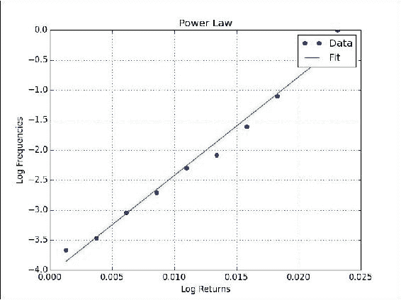
最后，我们将绘制数据并将其与 matplotlib 线性拟合：

plt.title('Power Law')
plt.plot(rets, freqs, 'o', label='Data')
plt.plot(rets, p[0] * rets + p[1], label='Fit')
plt.xlabel('Log Returns')
plt.ylabel('Log Frequencies')
plt.legend()
plt.grid()
plt.show()

我们得到一个很好的线性拟合，收益率和频率图，如下所示：

工作原理

histogram()函数计算数据集的直方图。它返回直方图值和桶的边界。 polyfit()函数将数据拟合给定阶数的多项式。在这种情况下，我们选择了线性拟合。我们发现了幂律法-您必须谨慎地提出此类主张，但证据看起来很有希望。

另见

第 1 章，“使用 IPython”中的“安装 matplotlib”秘籍
histogram()函数的文档页面
polyfit()函数的文档页面

逢低定期交易

股票价格周期性地下跌和上涨。我们将研究股价对数收益的概率分布，并尝试一个非常简单的策略。该策略基于对均值的回归。这是弗朗西斯·高尔顿爵士最初在遗传学中发现的一个概念。据发现，高大父母的孩子往往比父母矮。矮小父母的孩子往往比父母高。当然，这是一种统计现象，没有考虑基本因素和趋势，例如营养改善。均值回归也与股票市场有关。但是，它不提供任何保证。如果公司开始生产不良产品或进行不良投资，则对均值的回归将无法节省股票。

让我们首先下载股票的历史数据，例如AAPL。接下来，我们计算收盘价的每日对数回报率。我们将跳过这些步骤，因为它们在上一个秘籍中已经完成。

准备

如有必要，安装 matplotlib 和 SciPy。有关相应的秘籍，请参见“另请参见”部分。

操作步骤

以下是本书代码包中periodic.py文件的完整代码：

from __future__ import print_function
from matplotlib.finance import quotes_historical_yahoo
from datetime import date
import numpy as np
import scipy.stats
import matplotlib.pyplot as plt

#1\. Get close prices.
today = date.today()
start = (today.year - 1, today.month, today.day)

quotes = quotes_historical_yahoo('AAPL', start, today)
close =  np.array([q[4] for q in quotes])

#2\. Get log returns.
logreturns = np.diff(np.log(close))

#3\. Calculate breakout and pullback
freq = 0.02
breakout = scipy.stats.scoreatpercentile(logreturns, 100 * (1 - freq) )
pullback = scipy.stats.scoreatpercentile(logreturns, 100 * freq)

#4\. Generate buys and sells
buys = np.compress(logreturns < pullback, close)
sells = np.compress(logreturns > breakout, close)
print(buys)
print(sells)
print(len(buys), len(sells))
print(sells.sum() - buys.sum())

#5\. Plot a histogram of the log returns
plt.title('Periodic Trading')
plt.hist(logreturns)
plt.grid()
plt.xlabel('Log Returns')
plt.ylabel('Counts')
plt.show()

现在来了有趣的部分：

计算突破和回调。

假设我们要每年进行五次交易，大约每 50 天进行一次。一种策略是在价格下跌一定百分比时进行买入（回调），而在价格上涨另一百分比时进行卖出（突破）。

通过设置适合我们交易频率的百分比，我们可以匹配相应的对数回报。 SciPy 提供scoreatpercentile()函数，我们将使用：
```
freq = 0.02
breakout = scipy.stats.scoreatpercentile(logreturns, 100 * (1 - freq) )
pullback = scipy.stats.scoreatpercentile(logreturns, 100 * freq)
```
产生买卖。

使用compress() NumPy 函数为我们的收盘价数据生成买卖。该函数根据条件返回元素：
```
buys = np.compress(logreturns < pullback, close)
sells = np.compress(logreturns > breakout, close)
print(buys)
print(sells)
print(len(buys), len(sells))
print(sells.sum() - buys.sum())
```
AAPL和 50 天期间的输出如下：
```
[  77.76375466   76.69249773  102.72        101.2          98.57      ]
[ 74.95502967  76.55980292  74.13759123  80.93512599  98.22      ]
5 5
-52.1387025726
```
因此，如果我们买卖AAPL股票五次，我们将损失 52 美元。当我运行脚本时，经过更正后整个市场都处于恢复模式。您可能不仅要查看AAPL的股价，还可能要查看APL和SPY的比率。 SPY可以用作美国股票市场的代理。
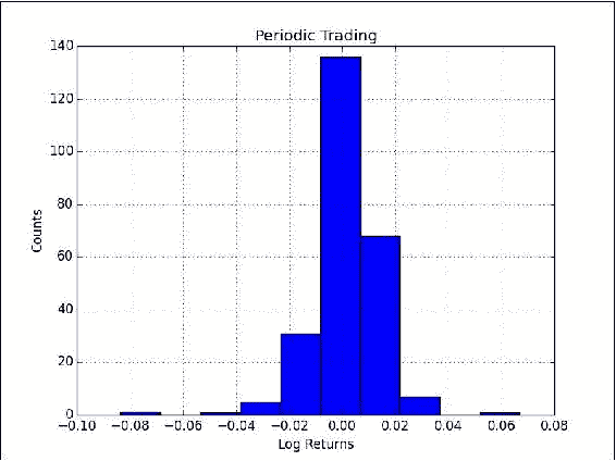
绘制对数回报的直方图。

只是为了好玩，让我们用 matplotlib 绘制对数回报的直方图：
```
plt.title('Periodic Trading')
plt.hist(logreturns)
plt.grid()
plt.xlabel('Log Returns')
plt.ylabel('Counts')
plt.show()
```
直方图如下所示：

工作原理

我们遇到了compress()函数，该函数返回一个数组，其中包含满足给定条件的输入的数组元素。输入数组保持不变。

另见

第 1 章，“使用 IPython”中的“安装 matplotlib”秘籍
第 2 章，“高级索引和数组概念”中的“安装 SciPy”秘籍
本章中的“发现幂律”秘籍
compress()函数文档页面

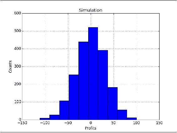
随机模拟交易

在先前的秘籍中，我们尝试了一种交易想法。但是，我们没有基准可以告诉我们所获得的结果是否良好。在这种情况下，通常以我们应该能够击败随机过程为前提进行随机交易。我们将从交易年度中随机抽出几天来模拟交易。这应该说明使用 NumPy 处理随机数。

准备

如有必要，安装 matplotlib。请参考相应秘籍的“另请参见”部分。

操作步骤

以下是本书代码包中random_periodic.py文件的完整代码：

from __future__ import print_function
from matplotlib.finance import quotes_historical_yahoo
from datetime import date
import numpy as np
import matplotlib.pyplot as plt

def get_indices(high, size):
   #2\. Generate random indices
   return np.random.randint(0, high, size)

#1\. Get close prices.
today = date.today()
start = (today.year - 1, today.month, today.day)

quotes = quotes_historical_yahoo('AAPL', start, today)
close =  np.array([q[4] for q in quotes])

nbuys = 5
N = 2000
profits = np.zeros(N)

for i in xrange(N):
   #3\. Simulate trades
   buys = np.take(close, get_indices(len(close), nbuys))
   sells = np.take(close, get_indices(len(close), nbuys))
   profits[i] = sells.sum() - buys.sum()

print("Mean", profits.mean())
print("Std", profits.std())

#4\. Plot a histogram of the profits
plt.title('Simulation')
plt.hist(profits)
plt.xlabel('Profits')
plt.ylabel('Counts')
plt.grid()
plt.show()

首先，我们需要一个数组，其中填充了随机整数：

生成随机索引。

您可以使用randint() NumPy 函数生成随机整数。这将与一个交易年度的随机日期相关联：
```
return np.random.randint(0, high, size)
```

模拟交易。

您可以使用上一步中的随机指数来模拟交易。使用take() NumPy 函数从步骤 1 的数组中提取随机收盘价：

buys = np.take(close, get_indices(len(close), nbuys))
sells = np.take(close, get_indices(len(close), nbuys))
profits[i] = sells.sum() - buys.sum()

绘制大量模拟的利润直方图：
```
plt.title('Simulation')
plt.hist(profits)
plt.xlabel('Profits')
plt.ylabel('Counts')
plt.grid()
plt.show()
```
以下是AAPL的 2,000 个模拟结果的直方图的屏幕截图，一年内进行了五次买卖：

工作原理

我们使用了randint()函数，该函数可以在numpy.random模块中找到。该模块包含更方便的随机生成器，如下表所述：

函数	描述
`rand()`	从`[0,1]`上的均匀分布中创建一个数组，其形状基于大小参数。如果未指定大小，则返回单个浮点数。
`randn()`	从均值`0`和方差`1`的正态分布中采样值。大小参数的作用与`rand()`相同。
`randint()`	返回一个给定下限，可选上限和可选输出形状的整数数组。

另见

第 1 章，“使用 IPython”中的“安装 matplotlib”秘籍

用 Eratosthenes 筛子筛选质数

Eratosthenes 筛子是一种过滤质数的算法。迭代地标识找到的质数的倍数。根据定义，倍数不是质数，可以消除。此筛子对于不到 1000 万的质数有效。现在让我们尝试找到第 10001 个质数。

操作步骤

第一步是创建自然数列表：

创建一个连续整数列表。 NumPy 为此具有arange()函数：
```
a = np.arange(i, i + LIM, 2)
```

筛选出p的倍数。

我们不确定这是否是 Eratosthenes 想要我们做的，但是它有效。在下面的代码中，我们传递 NumPy 数组，并去除除以p时余数为零的所有元素：

a = a[a % p != 0]

以下是此问题的完整代码：

from __future__ import print_function
import numpy as np

LIM = 10 ** 6
N = 10 ** 9
P = 10001
primes = []
p = 2

#By listing the first six prime numbers: 2, 3, 5, 7, 11, and 13, we can see that the 6th prime is 13.

#What is the 10 001st prime number?

def sieve_primes(a, p):
   #2\. Sieve out multiples of p
   a = a[a % p != 0]

   return a

for i in xrange(3, N, LIM):
   #1\. Create a list of consecutive integers
   a = np.arange(i, i + LIM, 2)

   while len(primes) < P:
      a = sieve_primes(a, p)
      primes.append(p)

      p = a[0]

print(len(primes), primes[P-1])

四、将 NumPy 与世界的其他地方连接

在本章中，我们将介绍以下秘籍：

使用缓冲区协议
使用数组接口
与 MATLAB 和 Octave 交换数据
安装 RPy2
与 R 交互
安装 JPype
将 NumPy 数组发送到 JPype
安装 Google App Engine
在 Google Cloud 上部署 NumPy 代码
在 PythonAnywhere Web 控制台中运行 NumPy 代码

简介

本章是关于互操作性的。我们必须不断提醒自己，NumPy 在科学（Python）软件生态系统中并不孤单。与 SciPy 和 matplotlib 一起工作非常容易。还存在用于与其他 Python 包互操作性的协议。在 Python 生态系统之外，Java，R，C 和 Fortran 等语言非常流行。我们将详细介绍与这些环境交换数据的细节。

此外，我们还将讨论如何在云上获取 NumPy 代码。这是在快速移动的空间中不断发展的技术。您可以使用许多选项，其中包括 Google App Engine 和 PythonAnywhere。

使用缓冲区协议

基于 C 的 Python 对象具有所谓的缓冲区接口。 Python 对象可以公开其数据以进行直接访问，而无需复制它们。缓冲区协议使我们能够与其他 Python 软件进行通信，例如 Python 图像库（PIL）。

我们将看到一个从 NumPy 数组保存 PIL 图像的示例。

准备

如有必要，请安装 PIL 和 SciPy。有关说明，查阅本秘籍的“另见”部分。

操作步骤

该秘籍的完整代码在本书代码包的buffer.py文件中：

import numpy as np
import Image #from PIL import Image (Python3)
import scipy.misc

lena = scipy.misc.lena()
data = np.zeros((lena.shape[0], lena.shape[1], 4), dtype=np.int8)
data[:,:,3] = lena.copy()
img = Image.frombuffer("RGBA", lena.shape, data, 'raw', "RGBA", 0, 1)
img.save('lena_frombuffer.png')

data[:,:,3] = 255 
data[:,:,0] = 222 
img.save('lena_modified.png')

首先，我们需要一个 NumPy 数组来玩：

在前面的章节中，我们看到了如何加载 Lena 的样例图像。创建一个填充零的数组，并使用图像数据填充 alpha 通道：
```
lena = scipy.misc.lena()
data = np.zeros((lena.shape[0], lena.shape[1], 4), dtype=numpy.int8)
data[:,:,3] = lena.copy()
```

使用 PIL API 将数据另存为 RGBA 图像：

img = Image.frombuffer("RGBA", lena.shape, data, 'raw', "RGBA", 0, 1)
img.save('lena_frombuffer.png')

通过去除图像数据并使图像变为红色来修改数据数组。使用 PIL API 保存图像：
```
data[:,:,3] = 255 
data[:,:,0] = 222 
img.save('lena_modified.png')
```
以下是之前的图片：

注意

在计算机图形中，原点的位置与您从高中数学中知道的通常的直角坐标系不同。原点位于屏幕，画布或图像的左上角，y 轴向下。

PIL 图像对象的数据由于缓冲接口的作用而发生了变化，因此，我们看到以下图像：

工作原理

我们从缓冲区（一个 NumPy 数组）创建了一个 PIL 图像。更改缓冲区后，我们看到更改反映在图像对象中。我们这样做时没有复制 PIL 图像对象；相反，我们直接访问并修改了其数据，以使模型的图片显示红色图像。通过一些简单的更改，代码就可以与其他基于 PIL 的库一起使用，例如 Pillow。

另见

第 2 章，“高级索引和数组概念”中的“安装 PIL”
第 2 章，“高级索引和数组概念”中的“安装 SciPy”
这个页面中介绍了 Python 缓冲区协议。

使用数组接口

数组接口是用于与其他 Python 应用通信的另一种机制。顾名思义，该协议仅适用于类似数组的对象。进行了示范。让我们再次使用 PIL，但不保存文件。

准备

我们将重用先前秘籍中的部分代码，因此前提条件是相似的。在这里，我们将跳过上一秘籍的第一步，并假定它已经为人所知。

操作步骤

该秘籍的代码在本书代码包的array_interface.py文件中：

from __future__ import print_function
import numpy as np
import Image
import scipy.misc

lena = scipy.misc.lena()
data = np.zeros((lena.shape[0], lena.shape[1], 4), dtype=np.int8)
data[:,:,3] = lena.copy()
img = Image.frombuffer("RGBA", lena.shape, data, 'raw', "RGBA", 0, 1)
array_interface = img.__array_interface__
print("Keys", array_interface.keys())
print("Shape", array_interface['shape'])
print("Typestr", array_interface['typestr'])

numpy_array = np.asarray(img)
print("Shape", numpy_array.shape)
print("Data type", numpy_array.dtype)

以下步骤将使我们能够探索数组接口：

PIL Image对象具有__array_interface__属性。让我们检查它的内容。此属性的值是 Python 字典：

array_interface = img.__array_interface__
print("Keys", array_interface.keys()) 
print("Shape", array_interface['shape'])
print("Typestr", array_interface['typestr'])

此代码显示以下信息：

Keys ['shape', 'data', 'typestr']
Shape (512, 512, 4)
Typestr |u1

NumPy ndarray类也具有__array_interface__属性。我们可以使用asarray()函数将 PIL 图像转换成 NumPy 数组：
```
numpy_array = np.asarray(img)
print("Shape", numpy_array.shape)
print("Data type", numpy_array.dtype)
```
数组的形状和数据类型如下：
```
Shape (512, 512, 4)
Data type uint8
```

如您所见，形状没有改变。

工作原理

数组接口或协议使我们可以在类似数组的 Python 对象之间共享数据。 NumPy 和 PIL 都提供了这样的接口。

另见

本章中的“使用缓冲区协议”
数组接口在这个页面中进行了详细描述。

与 MATLAB 和 Octave 交换数据

MATLAB 及其开放源代码 Octave 是流行的数学应用。 scipy.io包具有savemat()函数，该函数允许您将 NumPy 数组存储为.mat文件作为 Python 字典的值。

准备

安装 MATLAB 或 Octave 超出了本书的范围。 Octave 网站上有一些安装的指南。如有必要，检查本秘籍的“另见”部分，来获取安装 SciPy 的说明。

操作步骤

该秘籍的完整代码在本书代码包的octave.py文件中：

import numpy as np
import scipy.io

a = np.arange(7)

scipy.io.savemat("a.mat", {"array": a})

一旦安装了 MATLAB 或 Octave，就需要按照以下步骤存储 NumPy 数组：

创建一个 NumPy 数组，然后调用savemat()将其存储在.mat文件中。此函数有两个参数-文件名和包含变量名和值的字典。
```
a = np.arange(7)
scipy.io.savemat("a.mat", {"array": a})
```

导航到创建文件的目录。加载文件并检查数组：

octave-3.4.0:2> load a.mat
octave-3.4.0:3> array
array =

 0
 1
 2
 3
 4
 5
 6

另见

第 2 章，“高级索引和数组概念”中的“安装 SciPy”
savemat()函数的 SciPy 文档

安装 RPy2

R 是一种流行的脚本语言，用于统计和数据分析。 RPy2 是 R 和 Python 之间的接口。我们将在此秘籍中安装 RPy2。

操作步骤

如果要安装 RPy2，请选择以下选项之一：

使用pip或easy_install进行安装：RPy2 在 PYPI 上可用，因此我们可以使用以下命令进行安装：
```
$ easy_install rpy2
```
另外，我们可以使用以下命令：
```
$ sudo pip install rpy2
$ pip freeze|grep rpy2
rpy2==2.4.2
```

从源代码安装：我们可以从tar.gz源安装 RPy2：

$ tar -xzf <rpy2_package>.tar.gz
$ cd <rpy2_package>
$ python setup.py build install

另见

与 R 交互

RPy2 只能用作从 Python 调用 R，而不能相反。我们将导入一些样本 R 数据集并绘制其中之一的数据。

准备

如有必要，请安装 RPy2。请参阅先前的秘籍。

操作步骤

该秘籍的完整代码在本书代码包的rdatasets.py文件中：

from rpy2.robjects.packages import importr
import numpy as np
import matplotlib.pyplot as plt

datasets = importr('datasets')
mtcars = datasets.__rdata__.fetch('mtcars')['mtcars']

plt.title('R mtcars dataset')
plt.xlabel('wt')
plt.ylabel('mpg')
plt.plot(mtcars)
plt.grid(True)
plt.show()

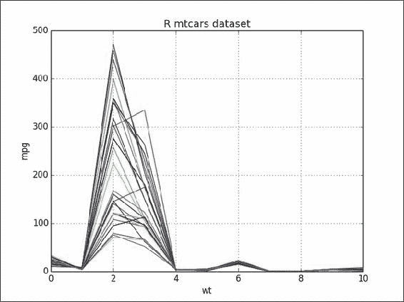
motorcars数据集在这个页面中进行了描述。让我们从加载此样本 R 数据集开始：

使用 RPy2 importr()函数将数据集加载到数组中。此函数可以导入R包。在此示例中，我们将导入数据集 R 包。从mtcars数据集创建一个 NumPy 数组：
```
datasets = importr('datasets')
mtcars = np.array(datasets.mtcars)
```
使用 matplotlib 绘制数据集：
```
plt.plot(mtcars)
plt.show()
```
数据包含英里每加仑（mpg）和重量（wt）值，单位为千分之一磅。以下屏幕快照显示了数据，它是一个二维数组：

另见

第 1 章“使用 IPython”中的“安装 matplotlib”

安装 JPype

Jython 是用于 Python 和 Java 的默认互操作性解决方案。但是，Jython 在 Java 虚拟机（JVM）上运行。因此，它无法访问主要用 C 语言编写的 NumPy 模块。 JPype 是一个开放源代码项目，试图解决此问题。接口发生在 Python 和 JVM 之间的本机级别上。让我们安装 JPype。

操作步骤

从这里下载 JPype。
打开压缩包，然后运行以下命令：
```
$ python setup.py install
```

将 NumPy 数组发送到 JPype

在此秘籍中，我们将启动 JVM 并向其发送 NumPy 数组。我们将使用标准 Java 调用打印接收到的数组。显然，您将需要安装 Java。

操作步骤

该秘籍的完整代码在本书代码包的hellojpype.py文件中：

import jpype
import numpy as np

#1\. Start the JVM
jpype.startJVM(jpype.getDefaultJVMPath())

#2\. Print hello world
jpype.java.lang.System.out.println("hello world")

#3\. Send a NumPy array
values = np.arange(7)
java_array = jpype.JArray(jpype.JDouble, 1)(values.tolist())

for item in java_array:
   jpype.java.lang.System.out.println(item)

#4\. Shutdown the JVM
jpype.shutdownJVM()

首先，我们需要从 JPype 启动 JVM：

从 JPype 启动 JVM； JPype 可以方便地找到默认的 JVM 路径：
```
jpype.startJVM(jpype.getDefaultJVMPath())
```
仅出于传统原因，让我们打印"hello world"：
```
jpype.java.lang.System.out.println("hello world")
```

创建一个 NumPy 数组，将其转换为 Python 列表，然后将其传递给 JPype。现在很容易打印数组元素：

values = np.arange(7)
java_array = jpype.JArray(jpype.JDouble, 1)(values.tolist())

for item in java_array:
    jpype.java.lang.System.out.println(item)

完成后，让我们关闭 JVM：
```
jpype.shutdownJVM()
```
JPype 中一次只能运行一个 JVM。如果我们忘记关闭 JVM，则可能导致意外错误。程序输出如下：
```
hello world
0.0
1.0
2.0
3.0
4.0
5.0
6.0
JVM activity report     :
 classes loaded       : 31
JVM has been shutdown
```

工作原理

JPype 允许我们启动和关闭 JVM。它为标准 Java API 调用提供了包装器。如本例所示，我们可以传递要由 JArray 包装器转换为 Java 数组的 Python 列表。 JPype 使用 Java 本机接口（JNI），这是本机 C 代码和 Java 之间的桥梁。不幸的是，使用 JNI 会损害性能，因此您必须注意这一事实。

另见

本章中的“安装 JPype”
JPype 主页

安装 Google App Engine

Google App Engine（GAE）使您可以在 Google Cloud 上构建 Web 应用。自 2012 年以来，是 NumPy 的官方支持；您需要一个 Google 帐户才能使用 GAE。

操作步骤

第一步是下载 GAE：

从这里下载适用于您的操作系统的 GAE。

您也可以从此页面下载文档和 GAE Eclipse 插件。 如果使用 Eclipse 开发，则一定要安装它。

开发环境。

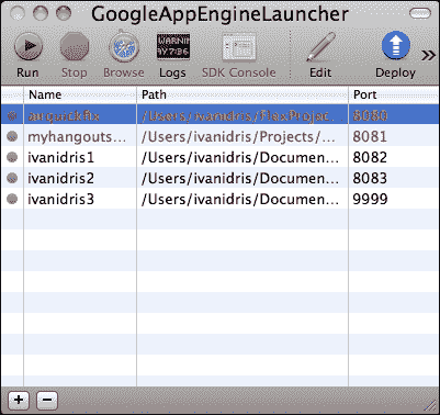
GAE 带有一个模拟生产云的开发环境。在撰写本书时，GAE 正式仅支持 Python 2.5 和 2.7。 GAE 将尝试在您的系统上找到 Python；但是，例如，如果您有多个 Python 版本，则可能需要自行设置。您可以在启动器应用的首选项对话框中设置此设置。

SDK 中有两个重要的脚本：
- dev_appserver.py：开发服务器
- appcfg.py：部署在云上
在 Windows 和 Mac 上，有一个 GAE 启动器应用。启动器具有运行和部署按钮，它们执行与上述脚本相同的操作。

在 Google Cloud 上部署 NumPy 代码

部署 GAE 应用非常容易。对于 NumPy，需要额外的配置步骤，但这仅需几分钟。

操作步骤

让我们创建一个新的应用：

使用启动器创建一个新应用（文件 | 新应用）。命名为numpycloud。这将创建一个包含以下文件的同名文件夹：
- app.yaml：YAML 应用配置文件
- favicon.ico：一个图标
- index.yaml：自动生成的文件
- main.py：Web 应用的主要入口点

将 NumPy 添加到库中。

首先，我们需要让 GAE 知道我们要使用 NumPy。将以下行添加到库部分中的app.yaml配置文件中：

- name: NumPy
  version: "1.6.1"

这不是最新的 NumPy 版本，但它是 GAE 当前支持的最新版本。配置文件应具有以下内容：

application: numpycloud
version: 1
runtime: python27
api_version: 1
threadsafe: yes

handlers:
- url: /favicon\.ico
  static_files: favicon.ico
  upload: favicon\.ico

- url: .*
  script: main.app

libraries:
- name: webapp2
  version: "2.5.1"
- name: numpy
  version: "1.6.1"

为了演示我们可以使用 NumPy 代码，让我们修改main.py文件。有一个MainHandler类，带有用于 GET 请求的处理器方法。用以下代码替换此方法：

def get(self):
    self.response.out.write('Hello world!<br/>')
    self.response.out.write('NumPy sum = ' + str(numpy.arange(7).sum()))

最后，我们将提供以下代码：

import webapp2
import numpy

class MainHandler(webapp2.RequestHandler):
    def get(self):
      self.response.out.write('Hello world!<br/>')
      self.response.out.write('NumPy sum = ' + str(numpy.arange(7).sum()))

app = webapp2.WSGIApplication([('/', MainHandler)],
                              debug=True)

如果您单击在 GAE 启动器中浏览按钮（在 Linux 上，以项目根为参数运行dev_appserver.py），则您应该在默认浏览器中看到一个包含以下文字的网页：

Hello world!NumPy sum = 21

工作原理

GAE 是免费的，具体取决于使用了多少资源。您最多可以创建 10 个 Web 应用。 GAE 采用沙盒方法，这意味着 NumPy 暂时无法使用，但现在可以使用，如本秘籍所示。

在 PythonAnywhere Web 控制台中运行 NumPy 代码

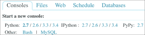
在第 1 章，“使用 IPython”中，我们已经看到了运行 PythonAnywhere 控制台的过程，而没有任何权限。此秘籍将需要您有一个帐户，但不要担心-它是免费的，如果您不需要太多资源，至少是免费的。

注册是一个非常简单的过程，此处将不涉及。 NumPy 已经与其他 Python 软件一起安装。有关完整列表，请参见这里。

我们将建立一个简单的脚本，该脚本每分钟从 Google 财经获取价格数据，并使用 NumPy 对价格进行简单的统计。

操作步骤

当我们签名后，我们可以登录并查看 PythonAnywhere 信息中心。

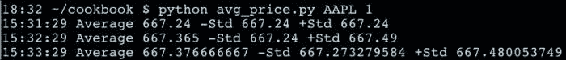
编写代码。此示例的完整代码如下：

from __future__ import print_function
import urllib2
import re
import time
import numpy as np

prices = np.array([])

for i in xrange(3):
   req = urllib2.Request('http://finance.google.com/finance/info?client=ig&q=AAPL')
   req.add_header('User-agent', 'Mozilla/5.0')
   response = urllib2.urlopen(req)
   page = response.read()
   m = re.search('l_cur" : "(.*)"', page)
   prices = np.append(prices, float(m.group(1)))
   avg = prices.mean()
   stddev = prices.std()

   devFactor = 1
   bottom = avg - devFactor * stddev
   top = avg + devFactor * stddev
   timestr = time.strftime("%H:%M:%S", time.gmtime())

   print(timestr, "Average", avg, "-Std", bottom, "+Std", top)
   time.sleep(60)

除我们在其中生长包含价格的 NumPy 数组并计算价格的均值和标准差的位以外，大多数都是标准 Python。如果有股票代号，例如AAPL，则可以使用 URL 从 Google 财经下载 JSON 格式的价格数据。该 URL 当然可以更改。

接下来，我们使用正则表达式解析 JSON 以提取价格。此价格已添加到 NumPy 数组中。我们计算价格的均值和标准差。价格是根据标准差乘以我们指定的某个因素后在时间戳的顶部和底部打印出来的。

上传代码。

在本地计算机上完成代码后，我们可以将脚本上传到 PythonAnywhere。转到仪表板，然后单击文件选项卡。从页面底部的小部件上传脚本。
要运行代码，请单击控制台选项卡，然后单击 Bash 链接。 PythonAnywhere 应该立即为我们创建一个 bash 控制台。现在，我们可以在一个标准差范围内运行AAPL程序，如以下屏幕截图所示：

工作原理

如果您想在远程服务器上运行 NumPy 代码，则 PythonAnywhere 是完美的选择，尤其是当您需要程序在计划的时间执行时。至少对于免费帐户而言，进行交互式工作并不那么方便，因为每当您在 Web 控制台中输入文本时都会有一定的滞后。

但是，正如我们所看到的，可以在本地创建和测试程序，并将其上传到 PythonAnywhere。这也会释放本地计算机上的资源。我们可以做一些花哨的事情，例如根据股价发送电子邮件或安排在交易时间内激活脚本。通过，使用 Google App Engine 也可以做到这一点，但是它是通过 Google 方式完成的，因此您需要了解其 API。

五、音频和图像处理

在本章中，我们将介绍 NumPy 和 SciPy 的基本图像和音频（WAV 文件）处理。在以下秘籍中，我们将使用 NumPy 对声音和图像进行有趣的操作：

将图像加载到内存映射中
添加图像
图像模糊
重复音频片段
产生声音
设计音频过滤器
使用 Sobel 过滤器进行边界检测

简介

尽管本书中的所有章节都很有趣，但在本章中，我们确实会继续努力并专注于获得乐趣。在第 10 章，“Scikits 的乐趣”中，您会发现更多使用scikits-image的图像处理秘籍。不幸的是，本书没有对音频文件的直接支持，因此您确实需要运行代码示例以充分了解其中的秘籍。

将图像加载到内存映射中

建议将大文件加载到内存映射中。内存映射文件仅加载大文件的一小部分。 NumPy 内存映射类似于数组。在此示例中，我们将生成彩色正方形的图像并将其加载到内存映射中。

准备

如有必要，“安装 matplotlib”的“另请参见”部分具有对相应秘籍的引用。

操作步骤

我们将通过初始化数组来开始：

首先，我们需要初始化以下数组：
- 保存图像数据的数组
- 具有正方形中心随机坐标的数组
- 具有平方的随机半径（复数个半径）的数组
- 具有正方形随机颜色的数组
初始化数组：
```
img = np.zeros((N, N), np.uint8)
NSQUARES = 30
centers = np.random.random_integers(0, N, size=(NSQUARES, 2))
radii = np.random.randint(0, N/9, size=NSQUARES)
colors = np.random.randint(100, 255, size=NSQUARES)
```
如您所见，我们正在将第一个数组初始化为零。其他数组使用numpy.random包中的函数初始化，这些函数生成随机整数。
下一步是生成正方形。我们在上一步中使用数组创建正方形。使用clip()函数，我们将确保正方形不会在图像区域外徘徊。 meshgrid()函数为我们提供了正方形的坐标。如果我们给此函数两个大小分别为N和M的数组，它将给我们两个形状为N x M的数组。第一个数组的元素将沿 x 轴重复。第二个数组将沿 y 轴重复其元素。以下示例 IPython 会话应该使这一点更加清楚：

注意
```
In: x = linspace(1, 3, 3)

In: x
Out: array([ 1.,  2.,  3.])
In: y = linspace(1, 2, 2)

In: y
Out: array([ 1.,  2.])

In: meshgrid(x, y)
Out:
[array([[ 1.,  2.,  3.],
 [ 1.,  2.,  3.]]),
 array([[ 1.,  1.,  1.],
 [ 2.,  2.,  2.]])]
```

最后，我们将设置正方形的颜色：

for i in xrange(NSQUARES):
   xindices = range(centers[i][0] - radii[i], centers[i][0] + radii[i])
   xindices = np.clip(xindices, 0, N - 1)
   yindices = range(centers[i][1] - radii[i], centers[i][1] + radii[i])
   yindices = np.clip(yindices, 0, N - 1)

   if len(xindices) == 0 or len(yindices) == 0:
      continue
   coordinates = np.meshgrid(xindices, yindices)
   img[coordinates] = colors[i]

在将图像数据加载到内存映射之前，我们需要使用tofile()函数将其存储在文件中。然后使用memmap()函数将图像文件中的图像数据加载到内存映射中：
```
img.tofile('random_squares.raw')
img_memmap = np.memmap('random_squares.raw', shape=img.shape)
```

为了确认一切正常，我们使用 matplotlib 显示图像：

plt.imshow(img_memmap)
plt.axis('off')
plt.show()

注意，我们没有显示轴。生成图像的示例如下所示：

这是本书代码包中memmap.py文件的完整源代码：

import numpy as np
import matplotlib.pyplot as plt

N = 512
NSQUARES = 30

# Initialize
img = np.zeros((N, N), np.uint8)
centers = np.random.random_integers(0, N, size=(NSQUARES, 2))
radii = np.random.randint(0, N/9, size=NSQUARES)
colors = np.random.randint(100, 255, size=NSQUARES)

# Generate squares
for i in xrange(NSQUARES):
   xindices = range(centers[i][0] - radii[i], centers[i][0] + radii[i])
   xindices = np.clip(xindices, 0, N - 1)
   yindices = range(centers[i][1] - radii[i], centers[i][1] + radii[i])
   yindices = np.clip(yindices, 0, N - 1)

   if len(xindices) == 0 or len(yindices) == 0:
      continue

   coordinates = np.meshgrid(xindices, yindices)
   img[coordinates] = colors[i]

# Load into memory map
img.tofile('random_squares.raw')
img_memmap = np.memmap('random_squares.raw', shape=img.shape)

# Display image
plt.imshow(img_memmap)
plt.axis('off')
plt.show()

工作原理

我们在此秘籍中使用了以下函数：

函数	描述
`zeros()`	此函数给出一个由零填充的数组。
`random_integers()`	此函数返回一个数组，数组中的随机整数值在上限和下限之间。
`randint()`	该函数与`random_integers()`函数相同，除了它使用半开间隔而不是关闭间隔。
`clip()`	该函数在给定最小值和最大值的情况下裁剪数组的值。
`meshgrid()`	此函数从包含 x 坐标的数组和包含 y 坐标的数组返回坐标数组。
`tofile()`	此函数将数组写入文件。
`memmap()`	给定文件名，此函数从文件创建 NumPy 内存映射。（可选）您可以指定数组的形状。
`axis()`	该函数是用于配置绘图轴的 matplotlib 函数。例如，我们可以将其关闭。

另见

第 1 章“使用 IPython”中的“安装 matplotlib”
NumPy 内存映射文档

合成图像

在此秘籍中，我们将结合著名的 Mandelbrot 分形和 Lena 图像。 Mandelbrot 集是数学家 Benoit Mandelbrot 发明的。这些类型的分形由递归公式定义，您可以在其中通过将当前拥有的复数乘以自身并为其添加一个常数来计算序列中的下一个复数。本秘籍将涵盖更多详细信息。

准备

如有必要，请安装 SciPy。“另请参见”部分具有相关秘籍的参考。

操作步骤

首先初始化数组，然后生成和绘制分形，最后将分形与 Lena 图像组合：

使用meshgrid()，zeros()和linspace()函数初始化对应于图像区域中像素的x，y和z数组：

x, y = np.meshgrid(np.linspace(x_min, x_max, SIZE),
                   np.linspace(y_min, y_max, SIZE))
c = x + 1j * y
z = c.copy()
fractal = np.zeros(z.shape, dtype=np.uint8) + MAX_COLOR

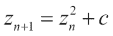
如果z是复数，则对于 Mandelbrot 分形具有以下关系：

在此，c是常数复数。这可以在复平面上绘制，水平轴显示实数值，垂直轴显示虚数值。我们将使用所谓的逃逸时间算法绘制分形。该算法以大约 2 个单位的距离扫描原点周围小区域中的点。这些点中的每一个都用作c值，并根据逃避区域所需的迭代次数为其指定颜色。如果所需的迭代次数超过了预定义的次数，则像素将获得默认背景色。有关更多信息，请参见此秘籍中已提及的维基百科文章：

for n in range(ITERATIONS):
    print(n)
    mask = numpy.abs(z) <= 4 
    z[mask] = z[mask] ** 2 +  c[mask]
    fractal[(fractal == MAX_COLOR) & (-mask)] = (MAX_COLOR - 1) * n / ITERATIONS
Plot the fractal with matplotlib:
plt.subplot(211)
plt.imshow(fractal)
plt.title('Mandelbrot')
plt.axis('off')
Use the choose() function to pick a value from the fractal or Lena array:
plt.subplot(212)
plt.imshow(numpy.choose(fractal < lena, [fractal, lena]))
plt.axis('off')
plt.title('Mandelbrot + Lena')

结果图像如下所示：

以下是本书代码集中mandelbrot.py文件中该秘籍的完整代码：

import numpy as np
import matplotlib.pyplot as plt
from scipy.misc import lena

ITERATIONS = 10
lena = lena()
SIZE = lena.shape[0]
MAX_COLOR = 255.
x_min, x_max = -2.5, 1
y_min, y_max = -1, 1

# Initialize arrays
x, y = np.meshgrid(np.linspace(x_min, x_max, SIZE),
                   np.linspace(y_min, y_max, SIZE))
c = x + 1j * y
z = c.copy()
fractal = np.zeros(z.shape, dtype=np.uint8) + MAX_COLOR
# Generate fractal
for n in range(ITERATIONS):
    mask = np.abs(z) <= 4 
    z[mask] = z[mask] ** 2 +  c[mask]
    fractal[(fractal == MAX_COLOR) & (-mask)] = (MAX_COLOR - 1) * n / ITERATIONS

# Display the fractal
plt.subplot(211)
plt.imshow(fractal)
plt.title('Mandelbrot')
plt.axis('off')

# Combine with lena
plt.subplot(212)
plt.imshow(np.choose(fractal < lena, [fractal, lena]))
plt.axis('off')
plt.title('Mandelbrot + Lena')

plt.show()

工作原理

在此示例中使用了以下函数：

函数	描述
`linspace()`	此函数返回范围内具有指定间隔的数字
`choose()`	此函数通过根据条件从数组中选择值来创建数组
`meshgrid()`	此函数从包含 x 坐标的数组和包含 y 坐标的数组返回坐标数组

另见

第 1 章，“使用 IPython”中的“安装 matplotlib”秘籍
第 2 章，“高级索引和数组”中的“安装 SciPy”秘籍

图像模糊

我们可以使用高斯过滤器来模糊图像。该过滤器基于正态分布。对应的 SciPy 函数需要标准差作为参数。在此秘籍中，我们还将绘制极地玫瑰和螺旋形。这些数字没有直接关系，但是在这里将它们组合起来似乎更有趣。

操作步骤

我们从初始化极坐标图开始，之后我们将模糊 Lena 图像并使用极坐标进行绘图：

初始化极坐标图：

NFIGURES = 5
k = np.random.random_integers(1, 5, NFIGURES)
a = np.random.random_integers(1, 5, NFIGURES)
colors = ['b', 'g', 'r', 'c', 'm', 'y', 'k']

要模糊 Lena，请应用标准差为4的高斯过滤器：

plt.subplot(212)
blurred = scipy.ndimage.gaussian_filter(lena, sigma=4)

plt.imshow(blurred)
plt.axis('off')

matplotlib 有一个polar()函数，它以极坐标进行绘制：

theta = np.linspace(0, k[0] * np.pi, 200)
plt.polar(theta, np.sqrt(theta), choice(colors))

for i in xrange(1, NFIGURES):
 theta = np.linspace(0, k[i] * np.pi, 200)
 plt.polar(theta, a[i] * np.cos(k[i] * theta), choice(colors))

这是这本书的代码集中spiral.py文件中该秘籍的完整代码：

import numpy as np
import matplotlib.pyplot as plt
from random import choice
import scipy
import scipy.ndimage
# Initialization
NFIGURES = 5
k = np.random.random_integers(1, 5, NFIGURES)
a = np.random.random_integers(1, 5, NFIGURES)

colors = ['b', 'g', 'r', 'c', 'm', 'y', 'k']

lena = scipy.misc.lena()
plt.subplot(211)
plt.imshow(lena)
plt.axis('off')

# Blur Lena
plt.subplot(212)
blurred = scipy.ndimage.gaussian_filter(lena, sigma=4)

plt.imshow(blurred)
plt.axis('off')

# Plot in polar coordinates
theta = np.linspace(0, k[0] * np.pi, 200)
plt.polar(theta, np.sqrt(theta), choice(colors))

for i in xrange(1, NFIGURES):
   theta = np.linspace(0, k[i] * np.pi, 200)
   plt.polar(theta, a[i] * np.cos(k[i] * theta), choice(colors))

plt.axis('off')

plt.show()

工作原理

在本教程中，我们使用了以下函数：

函数	描述
`gaussian_filter()`	此函数应用高斯过滤器
`random_integers()`	此函数返回一个数组，数组中的随机整数值在上限和下限之间
`polar()`	该函数使用极坐标绘制图形

另见

可以在这个页面中找到scipy.ndimage文档。

重复音频片段

正如我们在第 2 章，“高级索引和数组概念”中所看到的那样，我们可以使用 WAV 文件来完成整洁的事情。只需使用urllib2标准 Python 模块下载文件并将其加载到 SciPy 中即可。让我们下载一个 WAV 文件并重复 3 次。我们将跳过在第 2 章，“高级索引和数组概念”中已经看到的一些步骤。

操作步骤

尽管NumPy具有repeat()函数，但在这种情况下，更适合使用tile()函数。函数repeat()的作用是通过重复单个元素而不重复其内容来扩大数组。以下 IPython 会话应阐明这些函数之间的区别：
```
In: x = array([1, 2])

In: x
Out: array([1, 2])

In: repeat(x, 3)
Out: array([1, 1, 1, 2, 2, 2])

In: tile(x, 3)
Out: array([1, 2, 1, 2, 1, 2])
```
现在，有了这些知识，就可以应用tile()函数：
```
repeated = np.tile(data, 3)
```

使用 matplotlib 绘制音频数据：

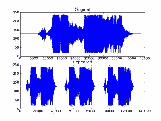
plt.title("Repeated")
plt.plot(repeated)

原始声音数据和重复数据图如下所示：

这是本书代码包中repeat_audio.py文件中该秘籍的完整代码：

import scipy.io.wavfile
import matplotlib.pyplot as plt
import urllib2
import numpy as np

response = urllib2.urlopen('http://www.thesoundarchive.com/austinpowers/smashingbaby.wav')
print(response.info())
WAV_FILE = 'smashingbaby.wav'
filehandle = open(WAV_FILE, 'w')
filehandle.write(response.read())
filehandle.close()
sample_rate, data = scipy.io.wavfile.read(WAV_FILE)
print("Data type", data.dtype, "Shape", data.shape)

plt.subplot(2, 1, 1)
plt.title("Original")
plt.plot(data)

plt.subplot(2, 1, 2)

# Repeat the audio fragment
repeated = np.tile(data, 3)

# Plot the audio data
plt.title("Repeated")
plt.plot(repeated)
scipy.io.wavfile.write("repeated_yababy.wav",
    sample_rate, repeated)

plt.show()

工作原理

以下是此秘籍中最重要的函数：

函数	描述
`scipy.io.wavfile.read()`	将 WAV 文件读入数组
`numpy.tile()`	重复数组指定次数
`scipy.io.wavfile.write()`	从 NumPy 数组中以指定的采样率创建 WAV 文件

另见

可以在这个页面中找到 scipy.io文档。

产生声音

声音可以用具有一定幅度，频率和相位的正弦波在数学上表示如下。我们可以从这个页面中指定的列表中随机选择符合以下公式的频率：

此处，n是钢琴键的编号。我们将键的编号从 1 到 88。我们将随机选择振幅，持续时间和相位。

操作步骤

首先初始化随机值，然后生成正弦波，编写旋律，最后使用 matplotlib 绘制生成的音频数据：

初始化随机值为：

200-2000之间的幅度
0.01-0.2的持续时间
使用已经提到的公式的频率

0和2 pi之间的相位值：

NTONES = 89
amps = 2000\. * np.random.random((NTONES,)) + 200.
durations = 0.19 * np.random.random((NTONES,)) + 0.01
keys = np.random.random_integers(1, 88, NTONES)
freqs = 440.0 * 2 ** ((keys - 49.)/12.)
phi = 2 * np.pi * np.random.random((NTONES,))

编写generate()函数以生成正弦波：

def generate(freq, amp, duration, phi):
 t = np.linspace(0, duration, duration * RATE)
 data = np.sin(2 * np.pi * freq * t + phi) * amp

 return data.astype(DTYPE)

一旦我们产生了一些音调，我们只需要组成一个连贯的旋律。现在，我们将连接正弦波。这不会产生良好的旋律，但可以作为更多实验的起点：
```
for i in xrange(NTONES):
   newtone = generate(freqs[i], amp=amps[i], duration=durations[i], phi=phi[i])
   tone = np.concatenate((tone, newtone))
```

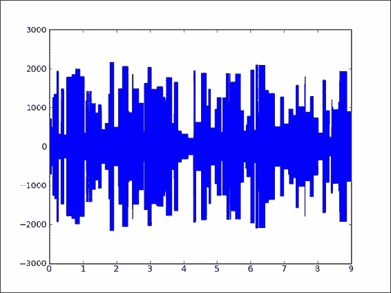
使用 matplotlib 绘制生成的音频数据：

plt.plot(np.linspace(0, len(tone)/RATE, len(tone)), tone)
plt.show()

生成的音频数据图如下：

可以在此处找到本示例的源代码，该代码来自本书代码包中的tone_generation.py文件：

import scipy.io.wavfile
import numpy as np
import matplotlib.pyplot as plt

RATE = 44100
DTYPE = np.int16

# Generate sine wave
def generate(freq, amp, duration, phi):
 t = np.linspace(0, duration, duration * RATE)
 data = np.sin(2 * np.pi * freq * t + phi) * amp

 return data.astype(DTYPE)

# Initialization
NTONES = 89
amps = 2000\. * np.random.random((NTONES,)) + 200.
durations = 0.19 * np.random.random((NTONES,)) + 0.01
keys = np.random.random_integers(1, 88, NTONES)
freqs = 440.0 * 2 ** ((keys - 49.)/12.)
phi = 2 * np.pi * np.random.random((NTONES,))

tone = np.array([], dtype=DTYPE) 

# Compose 
for i in xrange(NTONES):
   newtone = generate(freqs[i], amp=amps[i], duration=durations[i], phi=phi[i])
   tone = np.concatenate((tone, newtone))

scipy.io.wavfile.write('generated_tone.wav', RATE, tone)

# Plot audio data
plt.plot(np.linspace(0, len(tone)/RATE, len(tone)), tone)
plt.show()

工作原理

我们创建了带有随机生成声音的 WAV 文件。 concatenate()函数用于连接正弦波。

另见

concatenate()函数的文档

设计音频过滤器

我记得在模拟电子课上学习了所有类型的过滤器。然后，我们实际上构造了这些过滤器。可以想象，用软件制作过滤器要比用硬件制作过滤器容易得多。

我们将构建一个过滤器，并将其应用于要下载的音频片段。在本章之前，我们已经完成了一些步骤，因此我们将省略那些部分。

操作步骤

顾名思义，iirdesign()函数允许我们构造几种类型的模拟和数字过滤器。可以在scipy.signal模块中找到。该模块包含信号处理函数的完整列表：

使用scipy.signal模块的iirdesign()函数设计过滤器。 IIR 代表无限冲激响应；有关更多信息，请参见这里。我们将不涉及iirdesign())函数的所有细节。在这个页面中查看文档。简而言之，这些是我们将要设置的参数：
- 频率标准化为 0 到 1
- 最大损失
- 最小衰减
- 过滤器类型：
```
b,a = scipy.signal.iirdesign(wp=0.2, ws=0.1, gstop=60, gpass=1, ftype='butter')
```
此过滤器的配置对应于 Butterworth 过滤器。 Butterworth 过滤器由物理学家 Stephen Butterworth 于 1930 年首次描述。

使用scipy.signal.lfilter()函数应用过滤器。它接受上一步的值作为参数，当然也接受要过滤的数据数组：

filtered = scipy.signal.lfilter(b, a, data)

写入新的音频文件时，请确保其数据类型与原始数据数组相同：

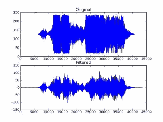
scipy.io.wavfile.write('filtered.wav', sample_rate, filtered.astype(data.dtype))

在绘制原始数据和过滤后的数据之后，我们得到以下图：

音频过滤器的代码列出如下：

import scipy.io.wavfile
import matplotlib.pyplot as plt
import urllib2
import scipy.signal

response =urllib2.urlopen('http://www.thesoundarchive.com/austinpowers/smashingbaby.wav')
print response.info()
WAV_FILE = 'smashingbaby.wav'
filehandle = open(WAV_FILE, 'w')
filehandle.write(response.read())
filehandle.close()
sample_rate, data = scipy.io.wavfile.read(WAV_FILE)
print("Data type", data.dtype, "Shape", data.shape)

plt.subplot(2, 1, 1)
plt.title("Original")
plt.plot(data)

# Design the filter
b,a = scipy.signal.iirdesign(wp=0.2, ws=0.1, gstop=60, gpass=1, ftype='butter')

# Filter
filtered = scipy.signal.lfilter(b, a, data)

# Plot filtered data
plt.subplot(2, 1, 2)
plt.title("Filtered")
plt.plot(filtered)

scipy.io.wavfile.write('filtered.wav', sample_rate, filtered.astype(data.dtype))

plt.show()

工作原理

我们创建并应用了 Butterworth 带通过滤器。引入了以下函数来创建过滤器：

函数	描述
`scipy.signal.iirdesign()`	创建一个 IIR 数字或模拟过滤器。此函数具有广泛的参数列表，该列表在这个页面中记录。
`scipy.signal.lfilter()`	给定一个数字过滤器，对数组进行滤波。

使用 Sobel 过滤器进行边界检测

Sobel 过滤器可以用于图像中的边界检测。边界检测基于对图像强度执行离散差分。由于图像是二维的，因此渐变也有两个分量，除非我们将自身限制为一维。我们将 Sobel 过滤器应用于 Lena 的图片。

操作步骤

在本部分中，您将学习如何应用 Sobel 过滤器来检测 Lena 图像中的边界：

要在 x 方向上应用 Sobel 过滤器，请将轴参数设置为0：
```
sobelx = scipy.ndimage.sobel(lena, axis=0, mode='constant')
```
要在 y 方向上应用 Sobel 过滤器，请将轴参数设置为1：
```
sobely = scipy.ndimage.sobel(lena, axis=1, mode='constant')
```

默认的 Sobel 过滤器仅需要输入数组：

default = scipy.ndimage.sobel(lena)

是原始图像图和所得图像图，显示了使用 Sobel 过滤器进行边界检测：

完整的边界检测代码如下：

import scipy
import scipy.ndimage
import matplotlib.pyplot as plt

lena = scipy.misc.lena()

plt.subplot(221)
plt.imshow(lena)
plt.title('Original')
plt.axis('off')

# Sobel X filter
sobelx = scipy.ndimage.sobel(lena, axis=0, mode='constant')

plt.subplot(222)
plt.imshow(sobelx)
plt.title('Sobel X')
plt.axis('off')

# Sobel Y filter
sobely = scipy.ndimage.sobel(lena, axis=1, mode='constant')

plt.subplot(223)
plt.imshow(sobely)
plt.title('Sobel Y')
plt.axis('off')

# Default Sobel filter
default = scipy.ndimage.sobel(lena)

plt.subplot(224)
plt.imshow(default)
plt.title('Default Filter')
plt.axis('off')

plt.show()

工作原理

我们将 Sobel 过滤器应用于著名模型 Lena 的图片。如本例所示，我们可以指定沿哪个轴进行计算。默认设置为独立于轴。

posted @ 2023-04-12 22:31 绝不原创的飞龙阅读(43) 评论(0) 收藏举报

刷新页面返回顶部

龙哥盟

掠夺·扩张·投机·博弈

NumPy 秘籍中文第二版：1~5

一、使用 IPython

简介

安装 IPython

操作步骤

工作原理

另见

使用 IPython 作为 Shell

操作步骤

工作原理

另见

阅读手册页

操作步骤

工作原理

安装 matplotlib

操作步骤

另见

运行 IPython 笔记本

准备

操作步骤

工作原理

另见

导出 IPython 笔记本

操作步骤

注意

导入网络笔记本

操作步骤

配置笔记本服务器

操作步骤

工作原理

另见

探索 SymPy 配置文件

准备

操作步骤

另见

二、高级索引和数组概念

简介

注意

安装 SciPy

准备

操作步骤

工作原理

另见

安装 PIL

操作步骤

另见

调整图像大小

注意

准备

操作步骤

工作原理

另见

创建视图和副本

准备

操作步骤

工作原理

另见

翻转 Lena

操作步骤

另见

花式索引

操作步骤

工作原理

另见

位置列表索引

操作步骤

另见

布尔值索引

操作步骤

工作原理

另见

数独的步幅技巧

注意

操作步骤

工作原理

另见

广播数组

操作步骤