SciTech-Mathmatics-Probability+Statistics: Assumptions, $\large P-value$, $\large overall\ F-value$ and $\large Null\ and\ Alternative\ Hypothesis$ for $\large Linear\ Regression\ Model$

Null and Alternative Hypothesis for Linear Regression

• Linear regression is a technique we can use to understand the relationship between one or more predictor variables and a response variable.

• To determine if there is a statistically significant relationship between a single predictor variable and the response variable, or to determine if there is a \(\large jointly\) statistically significant relationship between all predictor variables and the response variable, we need to analyze the \(\large overall\ F-value\) of the model and the corresponding \(\large P-value\).

• if the \(\large P-value\) is less than .05, we can reject the \(\large NH\).

Assumptions of Linear Regression

For the results of a LR(Linear Regression) model to be valid and reliable,
we need to check that the following four assumptions are met:

1. Linear relationship: There exists a linear relationship between the independent variable, x, and the dependent variable, y.
2. Independence: The residuals are independent. In particular, there is no correlation between consecutive residuals in time series data.
3. Homoscedasticity: The residuals have constant variance at every level of x.
4. Normality: The residuals of the model are normally distributed.

If one or more of these assumptions are violated, then the results of our linear regression may be unreliable or even misleading.

Refer to this post for:

• an explanation for each assumption,
• how to determine if the assumption is met,
• what to do if the assumption is violated.

Abbreviations

• \(\large SLR\) : \(\large Simple\ Linear\ Regression\)
• \(\large MLR\) : \(\large Multiple\ Linear\ Regression\)
• \(\large NH\) : \(\large Null\ Hypotheses\)
• \(\large AH\) : \(\large Alternative\ Hypotheses\)
• \(\large NAH\) : \(\large Null\ and\ Alternative\ Hypotheses\)

SLR(Simple Linear Regression)

If we only have one predictor variable and one response variable, we can use SLR(Simple Linear Regression), which uses the following formula to estimate the relationship between the variables:

\(\large \hat{y} = \beta_0+ \beta_1 x\)

• where:

  • \(\large \hat{y}\) : The estimated response value.
  • \(\large \beta_0\) : The average value of \(\large y\) when \(\large x\) is \(\large zero\).
  • \(\large \beta_1\) : The average change in \(\large y\) associated with a one unit increase in \(\large x\).
  • \(\large x\) : The value of the predictor variable.

• \(\large SLR\) uses the following \(\large NAH\):

  • \(\large H_0: \beta_1 = 0\)
  • \(\large H_A: \beta_1 \neq 0\)

• The \(\large Null\ Hypotheses\) states that the coefficient \(\large \beta_1\) is equal to zero.
  In other words, there is no statistically significant relationship between the predictor variable, \(\large x\), and the response variable, \(\large y\).

• The \(\large Alternative\ Hypotheses\) states that the coefficient \(\large \beta_1\) is not equal to zero. In other words, there is a statistically significant relationship between the predictor variable, \(\large x\), and the response variable, \(\large y\).

MLR(Multiple Linear Regression)

If we have multiple predictor variables and one response variable, we can use MLR(Multiple Linear Regression), which uses the following formula to estimate the relationship between the variables:

\(\large \hat{y} = \beta_0+ \beta_1 x_1 + \beta_2 x_2 + \cdots + \beta_k x_k\)

• where:

  • \(\large \hat{y}\) : The estimated response value.
  • \(\large \beta_0\) : The average value of \(\large y\) when all predictor variables are equal to \(\large zero\).
  • \(\large \beta_i\) : The average change in \(\large y\) associated with a one unit increase in \(\large x_i\).
  • $\large x_i $ : The value of the predictor variable $\large x_i $.

• \(\large MLR\) uses the following \(\large NAH\):

  • \(\large H_0: \beta_1 = \beta_2 = \cdots = \beta_k = 0\)
  • \(\large H_A: \beta_1 = \beta_2 = \cdots = \beta_k \neq 0\)

• The \(\large NH\) states that all coefficients in the model are equal to zero.
  In other words, none of the predictor variables $\large x_i $ have a statistically significant relationship with the response variable, \(\large y\).

• The \(\large alternative\ hypotheses\) states that not every coefficient is \(\large simultaneously\) equal to zero.

The following examples show how to decide to reject or fail to reject the \(\large NH\) in \(\large \text{ both }SLR \text{ and }MLR\) models.

Example 1: SLR(Simple Linear Regression)

Suppose a professor would like to use the number of hours studied to predict the exam score that students will receive in his class. He collects data for 20 students and fits a simple linear regression model.

The following screenshot shows the output of the regression model:

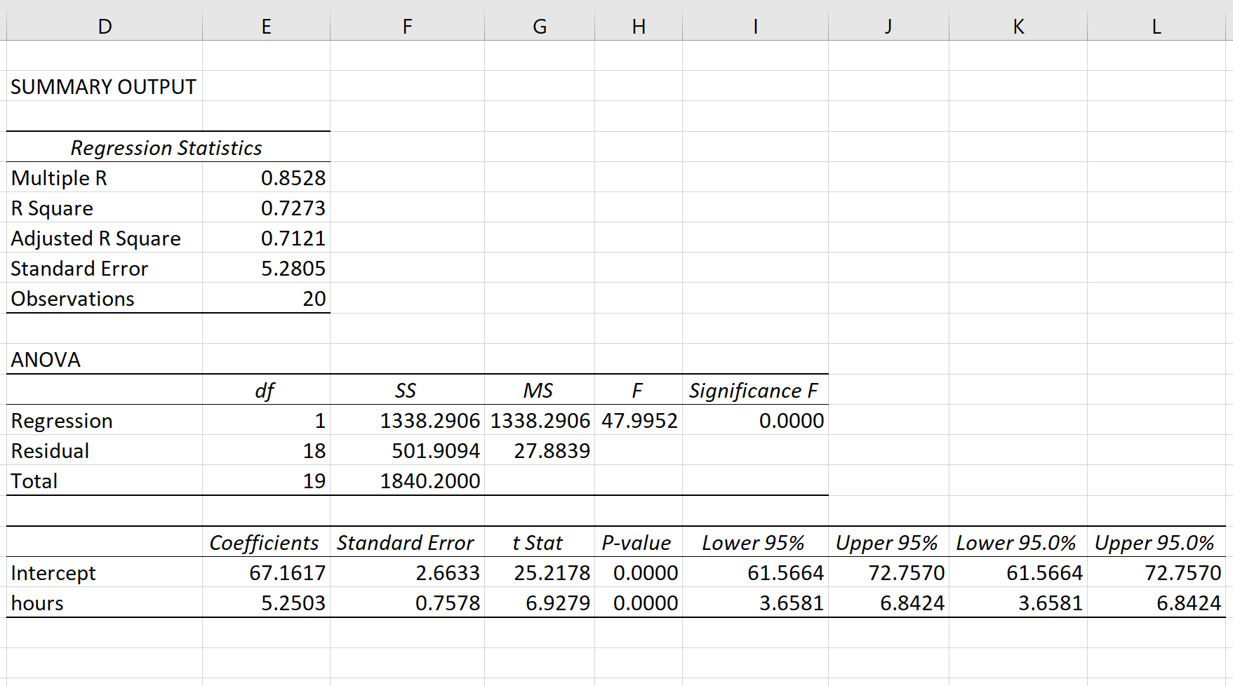
The fitted \(\large SLR\) model is:
$ Exam\ Score = 67.1617 + 5.2503*(hours\ studied)$

To determine if there is a statistically significant relationship between hours studied and exam score, we need to analyze the \(\large overall\ F-value\) of the model and the corresponding \(\large P-value\):

• \(\large Overall\ F-Value\) : 47.9952
• \(\large P-value\) : 0.000

Since this \(\large P-value\) is less than .05, we can reject the \(\large NH\).
In other words, there is a statistically significant relationship between hours studied and exam score received.

Example 2: MLR(Multiple Linear Regression)

Suppose a professor would like to use the number of hours studied and the number of prep exams taken to predict the exam score that students will receive in his class. He collects data for 20 students and fits a multiple linear regression model.
The following screenshot shows the output of the regression model(\(\large MLR\) output in Excel):

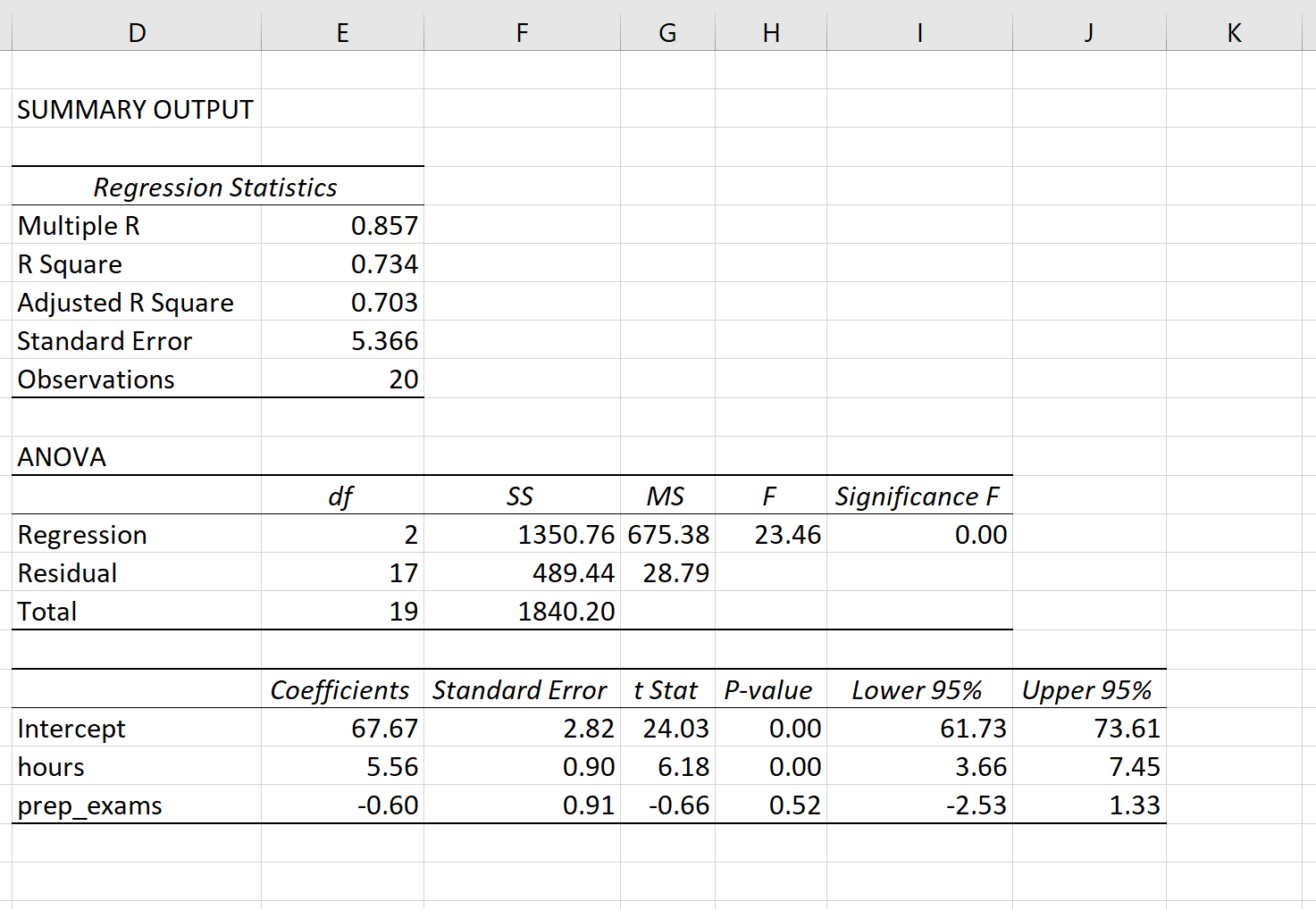
The fitted \(\large MLR\) model is:
\(Exam\ Score = 67.67 + 5.56*(hours\ studied) – 0.60*(prep\ exams\ taken)\)

To determine if there is a \(\large jointly\) statistically significant relationship between the two predictor variables and the response variable, we need to analyze the \(\large Overall\ F-Value\) of the model and the corresponding \(\large P-value\):

• \(\large Overall\ F-Value\) : 23.46
• \(\large P-value\) : 0.00

Since this \(\large P-value\) is less than .05, we can reject the \(\large NH\).
In other words, hours studied and prep exams taken have a jointly statistically significant relationship with exam score.

Note: Although the \(\large P-value\) for prep exams taken (p = 0.52) is not significant, prep exams combined with hours studied has a significant relationship with exam score.

Additional Resources

Understanding the F-Test of Overall Significance in Regression
How to Read and Interpret a Regression Table
How to Report Regression Results
How to Perform Simple Linear Regression in Excel
How to Perform Multiple Linear Regression in Excel