
SciTech-BigDataAI-ImageProcessing-OpenCV-Edge Detection(边缘检测) + Background Subtraction(背景差分过阈值) Methods + NumPy + Pandas
https://docs.opencv.org/3.4/d1/dc5/tutorial_background_subtraction.html
总结
OpenCV 提供了多种有效的边缘检测方法,能够满足不同的图像处理需求。
通过理解每种算法的原理和参数调整,可以在各种图像处理应用中灵活运用边缘检测技术。
边缘检测在对象检测、图像分割、特征提取等领域都有广泛的应用.
掌握这些基本方法能为更高级的图像处理打下基础。
边缘检测与轮廓检测的区别
OpenCV 的边缘检测和轮廓检测虽然都与图像的形状和边界有关,
但它们有明显的区别:
Edge边缘:
https://www.geeksforgeeks.org/python/real-time-edge-detection-using-opencv-python/
https://coderivers.org/opencv/opencv-image-edge-detection/
Contour轮廓:
https://docs.opencv.org/3.4/d4/d73/tutorial_py_contours_begin.html
- 边缘检测
- 目标:
找出图像上亮度变化明显的像素点,即图像的边缘。 - 方法:
使用各种边缘检测算子,如Canny、Sobel、Laplacian等,这些算子利用图像的梯度信息判断边缘。 - 输出: 一张边缘图像,
标记出边缘像素点,通常为黑白图像。 - 应用: 提取图像的轮廓信息、用于图像分割、特征提取
- 目标:
- 轮廓检测
- 目标:
找到图像上闭合的曲线,即物体的轮廓。 - 方法:
使用 findContours() 函数,该函数会提取出所有闭合的轮廓,并返回其列表形式。 - 输出: 一个轮廓列表,每个轮廓
包含一个点集,这些点集代表轮廓的坐标。 - 应用: 识别物体形状、测量物体大小和面积、物体计数、物体跟踪
- 目标:
区别总结:
| 特征 | 边缘检测 | 轮廓检测 |
|---|---|---|
| 定义 | 在图像上画线,标记出边缘的位置 | 就像是在图像上描边,将物体完整地勾勒出来 |
| 目标 | 找到图像上的边缘点(亮度变化明显的像素点) | 找到图上的闭合轮廓(闭合的曲线) |
| 方法 | 使用边缘检测算子 | 使用 findContours() 函数 |
| 输出 | 边缘图像 | 轮廓列表 |
| 应用 | 轮廓提取、图像分割、特征提取 | 物体识别、测量、计数、跟踪 |
举例:
如果你想要检测一张照片的人物轮廓,
可以使用 边缘检测 找到人物边缘,
然后使用 轮廓检测 将人物轮廓完整地提取出。
需要注意的是:
边缘检测的结果可以作为轮廓检测的输入。
在实际应用上,边缘检测和轮廓检测往往会结合使用,以达到更好的效果。
Edge Detection(边缘检测)
参考 :
Background Removal with Python
Using OpenCV to Detect the Foreground
https://towardsdatascience.com/background-removal-with-python-b61671d1508a/
-
Laplacian(拉普拉斯算子):
cv2.Laplacian函数
"二阶导数"算子, 用于图像的Edge Detection
它通过计算图像的 “二阶导数”来检测“强烈变化的区域(边缘)” -
Sobel算子: 使用
cv2.Sobel函数
使用cv2.Sobel函数对图像进行处理
"一阶导数"算子,用于图像的Edge Detection, 分别计算 x方向 和 y方向 的边缘信号.- sobelx("x方向上的 Sobel算子") 检测 "垂直的边缘",显示 "水平边"
- sobely("y方向上的 Sobel算子") 检测 "水平的边缘",显示 "垂直边"
-
Canny 算子:
cv2.Canny函数
import cv2 as cv
import numpy as np
from matplotlib import pyplot as plt
img0 = cv.imread('./data/Signature.jpg', 0)
edges0 = cv.Canny(img0, 100, 20)
# Canny函数的参数(两个阈值):
# * threshold1: 低阈值, "像素点值<此阈值" 时, 跳过(不是边缘)。
# * threshold2: 高阈值, "像素点值>此阈值" 时, 存续(判定边缘)。
# 怎么选取最优的 两个参数阈值? 参看后文:
cv.imwrite("Edges0.png", edges0)
# This step is strictly optional, but dilating and eroding the edges,
# make them more pronounced and returns a nicer final product.
edges0 = cv.dilate(edges0, None)
edges0 = cv.erode(edges0, None)
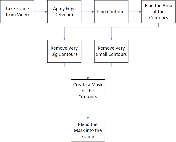
# get the contours and their areas
contours = cv.findContours(edges0, cv.RETR_LIST, cv.CHAIN_APPROX_NONE)
contour_info = [(c, cv.contourArea(c),) for c in contours[1] ]
cv.imshow('Edges', edges0)
cv.waitKey(0)
OpenCV 直方统计+ 直方均衡化
直方图均衡化 和 规定化 是 数字图像处理 常用的两种方法,它们的目的和区别如下:
- Histogram Equalization(直方图均衡化)
目的: "增强对比度",使图像 的"细节更加明显"。
基本思想:调整像素值,使"像素值分布"更加均匀, 达到提升动态范围。
适用: "像素值分布不均匀" 的图,例如 "低对比度的图"。 - Specification(规定化):
目的: 使 一张图 "像素值分布" 和另一张图 的 "像素值分布" 相同。
基本思想:调整像素值, 使其 "像素值分布" 与 目标图 的 "像素值分布"相同。
适用: 调整 多张图 在 同一特征 上的 像素值分布 成为 相同。常用在 色调, 饱和度, 亮度 等特征上。 - Hist.Equ. 与 Spe. 的区别:
Hist.Equ. 调整 "像素值分布"的方式 是 使得 "像素值均匀分布"
Spe. 调整 "像素值分布"的方式 是 将其调整为 "目标分布",进一步 实现 多图像 的同一特征 对比 与 转换。 - 直方图均衡化 和 规定化 常用于 图像增强、图像分类、目标检测等领域。例如,
利用 Hist.Equ. 作 图像增强,使得 "目标特征" 更加明显;
利用 Spe. 将 多张图 在 "同一特征(例如对比度)" 上调整 "像素值分布" 为相同, 以实现多图的 融合和匹配。
背景
- 像素分布(分析整张图片的): 是 图像处理 经常要先统计出,为进一步的处理提供决策数据。
- 图片 与 (特征)直方数据 是 "多对一" 的映射关系:
任一幅图,都有其唯一的一幅"(特征)直方数据"。
不同的图,可能有相同的"(特征)直方数据"。 - 直方数据: 是统计学上一种常用的统计 "数据分布 "的过程:
- 先统计出"直方数据",后作"二维图表"可视化。
- 两个坐标,分别是 "统计样本(图像、视频帧)" 和 "样本的一种特征",
如 像素值, 灰度值, 亮度, 梯度, 方向, 色彩, 等任何特征.
- 像素值 的 直方数据:
统计出 “所有的像素值” 及 “每个像素值的出现个数” :- "x轴点集" 是 "所有的像素值(图片有的, 升序)",
- 一个"y轴值(像素个数)" 对应一个“x轴点”
- 借助 "直方数据" 观察要如何调整“像素值分布”。
横坐标 的 左侧为 纯黑、较暗的区域,而右侧为较亮、纯白的区域。
"直方数据" 多集中在 "左侧和中间"则原图 "较暗",反之则"较亮"。
- 灰度值 的 直方数据:
一幅图像 的 "像素灰度值" 的 "出现次数(或频数)" 的 统计结果。
它只反映 灰度值 的 "像素频率(出现概率)",而未反映 "一灰度值" 的 "像素所在位置"。 - CV(计算机视觉)常借助 直方数据 来实现图像的高智能全自动化处理。
直方统计: cv2.calcHist()
OpenCV 使用 cv2.calcHist() 函数原型:
hist = cv2.calcHist(images, channels, mask, histSize, ranges, accumulate)
参数含义如下:
images: 输入图channels: 指定通道
"通道编号" 要用 "[]"括起来.
灰度图(只有一个channel)时, 值为"[0]".
彩色图用[0], [1] 或 [2] 分别对应通道 B,G,R。mask: 掩码图
统计 "整幅图",设为None。
统计 "部分图",要传 "mask". 生成 "图的mask"示例:
mask = np.zeros(image.shape, np.uint8)
mask[200:400, 200:400] = 255histSize: BINS的数量(横轴点数量)ranges: 纵轴值RANGE(纵轴点值范围)
纵轴值 的 范围,例如:对像素值 特征常为[0, 255],accumulate: 累计标识, 默认值 为false,
如果设置为true,则直方数据 在 开始分配 时, 不会被清零.
该参数允许对 "多个对象" 计算 "总体的直方数据",
或用户实施更新 "直方数据"( 多份"增量数据"的累计结果).return value: hist : 直方数据
直方均衡化: cv2.equalizeHist(src[, dst])
直方均衡化 的数学原理 是 映射 "一个分布(输入数据) 到 "另一个分布(一个更理想统一的分布).
函数原型
dst = cv2.equalizeHist(src[, dst])
- 参数含义:
src: 单通道 8-bit 的图像dst: 与 输入图 大小相同的 输出图
- 函数实现: 对 输入图 作 直方均衡化:
对 直方数据 的 "每个灰度级" 进行 "normalization"处理,
统计 "每种灰度" 的 "累积分布",得到一个 灰度映射表,
然后, 根据 "其灰度值" 来 修正原图的 "每个像素"。
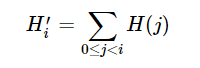
过程大概是:- 计算 输入图 的 直方数据 H;
- 直方normalization化,使不同 bins 的 直方数据 和为 255;
- 计算 直方数据 积分:
![]()
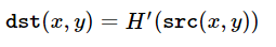
- 以 H' 作为查询表进行图像变换:
![]()
直方图 示例 及 源码
| 原图 | 灰度值 直方图 | RGB 直方图 | mask 的直方图 |
|---|---|---|---|
 |
 |
 |
 |
import cv2
import matplotlib
import matplotlib.pyplot as plt
import numpy as np
# 在服务端调试不显示
matplotlib.use('Agg')
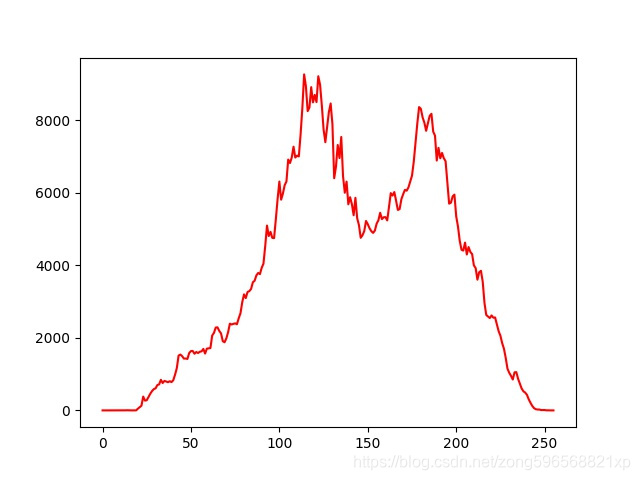
# 灰度值 直方图
def calchist_for_gray(imgname):
img = cv2.imread(imgname, cv2.IMREAD_GRAYSCALE)
hist = cv2.calcHist([img], [0], None, [256], [0, 255])
plt.plot(hist, color="r"); plt.savefig("result_gray.jpg")
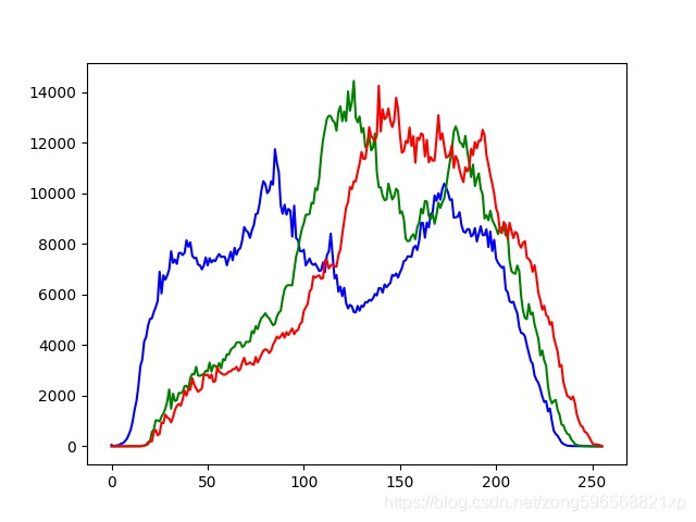
# RGB 直方图
def calchist_for_rgb(img_path):
img = cv2.imread(img_path)
histb = cv2.calcHist([img], [0], None, [256], [0, 255])
histg = cv2.calcHist([img], [1], None, [256], [0, 255])
histr = cv2.calcHist([img], [2], None, [256], [0, 255])
plt.plot(histb, color="b"); plt.plot(histg, color="g"); plt.plot(histr, color="r")
plt.savefig("result_rgba.jpg")
# 生成 image 的 mask image
def get_mask(img_path):
image = cv2.imread(img_path, 0)
mask = np.zeros(image.shape, np.uint8)
mask[200:400, 200:400] = 255
mi = cv2.bitwise_and(image, mask)
cv2.imwrite("mi.jpg", mi)
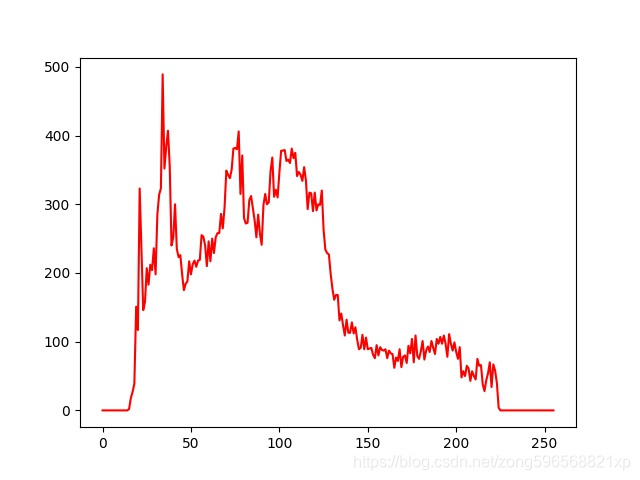
# mask 的直方图
def calchist_for_mask(imgname):
img = cv2.imread(imgname, cv2.IMREAD_GRAYSCALE)
mask = np.zeros(img.shape, np.uint8)
mask[200:400, 200:400] = 255
histMI = cv2.calcHist([img], [0], mask, [256], [0, 255])
histImage = cv2.calcHist([img], [0], None, [256], [0, 255])
plt.plot(histMI, color="r"); plt.savefig("result_mask.jpg")
# plt.show()
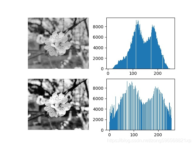
# 直方均衡化
def get_equalizehist_img(imgname):
    img = cv2.imread(imgname, cv2.IMREAD_GRAYSCALE)
    equ = cv2.equalizeHist(img)

    plt.subplot(221); plt.imshow(img, plt.cm.gray); plt.axis('off')
    plt.subplot(222); plt.hist(img.ravel(), 256)

    plt.subplot(223); plt.imshow(equ, plt.cm.gray); plt.axis('off')
    plt.subplot(224); plt.hist(equ.ravel(), 256)
    plt.savefig("result2.jpg")
How to Use Background Subtraction Methods
Next Tutorial: Meanshift and Camshift
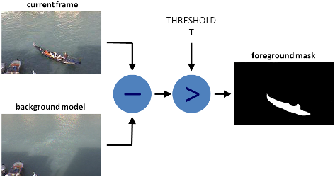
- Background subtraction (BS) is a common and widely used technique for generating a foreground mask (namely, a binary image containing the pixels belonging to moving objects in the scene) by using static cameras.
- As the name suggests, BS calculates the foreground mask performing a subtraction between the current frame and a background model, containing the static part of the scene or, more in general, everything that can be considered as background given the characteristics of the observed scene.
Background_Subtraction_Tutorial_Scheme.png
![]()
- Background modeling consists of two main steps:
- Background Initialization;
In the first step, "an initial model" of the background is computed, - Background Update.
In the second step, that model is updated in order to adapt to possible changes in the scene.
- Background Initialization;
- In this tutorial we will learn how to perform BS by using OpenCV.
Goals
In this tutorial you will learn how to:
- Read data from videos or image sequences by using cv::VideoCapture ;
- Create and update the background model by using cv::BackgroundSubtractor class;
- Get and show the foreground mask by using cv::imshow ;
Code
In the following you can find the source code.
We will let the user choose to process either a video file or a sequence of images.
We will use cv::BackgroundSubtractorMOG2 in this sample, to generate the foreground mask.
The results as well as the input data are shown on the screen.
Downloadable code: Click here
Code at glance:
from __future__ import print_function
import cv2 as cv
import argparse
parser = argparse.ArgumentParser(description='This program shows how to use background subtraction methods provided by OpenCV. You can process both videos and images.')
parser.add_argument('--input', type=str, help='Path to a video or a sequence of image.', default='vtest.avi')
parser.add_argument('--algo', type=str, help='Background subtraction method (KNN, MOG2).', default='MOG2')
args = parser.parse_args()

if args.algo == 'MOG2':
    backSub = cv.createBackgroundSubtractorMOG2()
else:
    backSub = cv.createBackgroundSubtractorKNN()

capture = cv.VideoCapture(cv.samples.findFileOrKeep(args.input))
if not capture.isOpened():
    print('Unable to open: ' + args.input)
    exit(0)

while True:
    ret, frame = capture.read()
    if frame is None:
        break
    fgMask = backSub.apply(frame)
    cv.rectangle(frame, (10, 2), (100,20), (255,255,255), -1)
    cv.putText(frame, str(capture.get(cv.CAP_PROP_POS_FRAMES)), (15, 15),
               cv.FONT_HERSHEY_SIMPLEX, 0.5 , (0,0,0))

    cv.imshow('Frame', frame)
    cv.imshow('FG Mask', fgMask)

    keyboard = cv.waitKey(30)
    if keyboard == 'q' or keyboard == 27:
        break
Explanation
We discuss the main parts of the code above:
- A cv::BackgroundSubtractor object will be used to generate the foreground mask. In this example, default parameters are used, but it is also possible to declare specific parameters in the create function.
#create Background Subtractor objects
if args.algo == 'MOG2':
    backSub = cv.createBackgroundSubtractorMOG2()
else:
    backSub = cv.createBackgroundSubtractorKNN()
- A cv::VideoCapture object is used to read the input video or input images sequence.
capture = cv.VideoCapture(cv.samples.findFileOrKeep(args.input))
if not capture.isOpened():
    print('Unable to open: ' + args.input)
    exit(0)
- Every frame is used both for calculating the foreground mask and for updating the background. If you want to change the learning rate used for updating the background model, it is possible to set a specific learning rate by passing a parameter to the apply method.
    #update the background model
    fgMask = backSub.apply(frame)
- The current frame number can be extracted from the cv::VideoCapture object and stamped in the top left corner of the current frame. A white rectangle is used to highlight the black colored frame number.
    #get the frame number and write it on the current frame
    cv.rectangle(frame, (10, 2), (100,20), (255,255,255), -1)
    cv.putText(frame, str(capture.get(cv.CAP_PROP_POS_FRAMES)), (15, 15),
               cv.FONT_HERSHEY_SIMPLEX, 0.5 , (0,0,0))
- We are ready to show the current input frame and the results.
    #show the current frame and the fg masks
    cv.imshow('Frame', frame)
    cv.imshow('FG Mask', fgMask)
Results
-
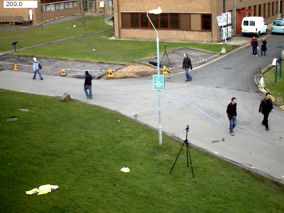
With the vtest.avi video, for the following frame:
![]()
Background_Subtraction_Tutorial_frame.jpg -
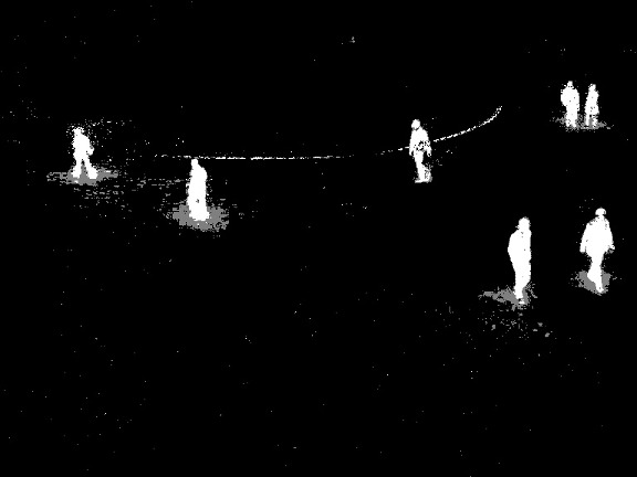
The output of the program will look as the following for the MOG2 method (gray areas are detected shadows):
![]()
Background_Subtraction_Tutorial_result_MOG2.jpg -
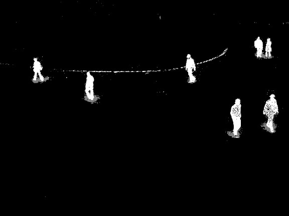
The output of the program will look as the following for the KNN method (gray areas are detected shadows):
![]()
Background_Subtraction_Tutorial_result_KNN.jpg
References
- Background Models Challenge (BMC) website
- A Benchmark Dataset for Foreground/Background Extraction [221]

 浙公网安备 33010602011771号