【概率论与数理统计】小结8 - 三大抽样分布以及p值的计算
注:抽样分布就是统计量的分布,其特点是不包含未知参数且尽可能多的概括了样本信息。除了常见的正态分布之外,还有卡方分布、t分布和F分布为最常见的描述抽样分布的分布函数。这几个分布函数在数理统计中也非常有名。我们常说的卡方检验、t检验和F检验就跟这三个分布有关。下面分别从定义、性质、函数图像和分位数等方面介绍三大分布。
0. 分位点/分位数(Fractile)
分位数是一个非常重要的概念,一开始也有点难理解。首先要明确一点,分位数分的是面积。更准确的说,分位数分的是某个特定分布的概率密度函数曲线下的面积。每给定一个分位数,这个概率密度函数曲线就被该点一分为二。
在英语中,表示分位数的有两个词,它们的区别如下:
As nouns the difference between fractile and quantile is that fractile is (statistics) the value of a distribution for which some fraction of the sample lies below while quantile is (statistics) one of the class of values of a variate which divides the members of a batch or sample into equal-sized subgroups of adjacent values or a probability distribution into distributions of equal probability.
摘自,https://wikidiff.com/fractile/quantile
因此,从上面的描述可以看出来这里所说的分位点是指fractile。其实还有一个词,percentile,这个词好像用的更多。
四分位数(Quartiles)
四分位数是平时用的比较多的概念,属于quantile的一种。对于一组数据来说,四分位数就是将这组数据排序后,均分为4部分的3个分割点位置的数值。例如1, 3, 5, 7, 9, 11,其3个四分位点分别是3,6,9。分别叫做第一四分位数(Q1),第二四分位数(Q2),第三四分位数(Q3)。
对于概率密度函数来说,四分位点就是将概率密度曲线下的面积均分为4部分的点。
上$\alpha$分位数(Upper Percentile)
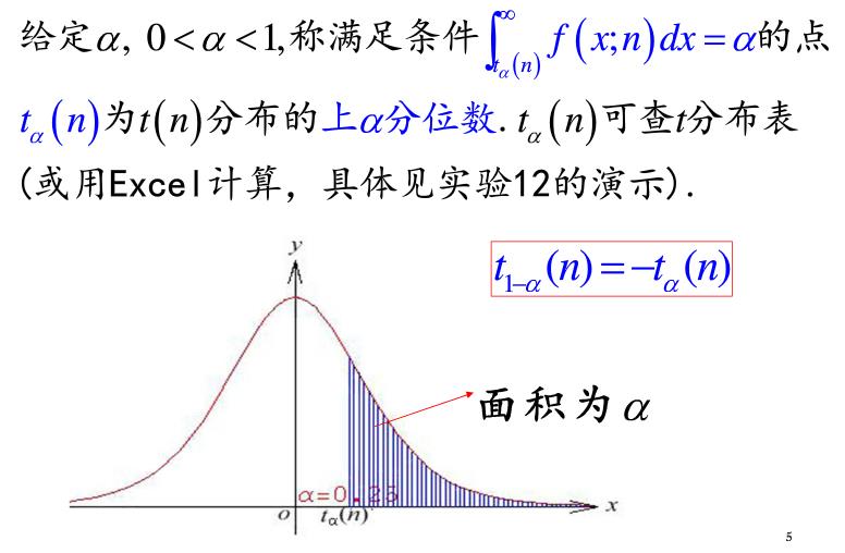
上$\alpha$分位数是概率密度函数定义域内的一个数值,这个数值将概率密度函数曲线下的面积沿x轴分成了两个部分,其中该点右侧部分概率密度函数曲线与x轴围成的面积等于$\alpha$。

图1,某分布的上$\alpha$分位数,$x_{\alpha}$
由于概率密度函数曲线下的面积就是概率,因此上$\alpha$分位数中的$\alpha$就是该点右侧区域的面积(图1红色区域),也是在这个分布中取到所有大于该点的值的概率。在假设检验中这个概率就是我们通常说的P值。
参考图1,$P(X \geq x_{\alpha}) = \alpha$
此时有两个值,一个是$\alpha$,另一个是$x_{\alpha}$。这两个值中确定其中一个,另一个值也就确定了。因此我们可以通过一个给定的$\alpha$值,求在某个特定分布中的上$\alpha$分位数,即$x_{\alpha}$,的值;也可以在某个特定分布中,任意给定一个定义域内的点$x_1$,求取到比该点的值更大的值的概率,即$P(X \geq x_1)$的值。
1. 卡方分布($\chi^2$)
从其名称中可以看到,卡方分布跟平方有关。事实也是这样,卡方分布是由服从标准正态分布的随机变量的平方和组成的。
1.1 定义
设随机变量 $X_1, X_2, ..., X_n$ 相互独立,都服从 $N(0, 1)$,则称
$$\chi^2 = \displaystyle \sum_{ i = 1 }^{ n } X_i^2$$
服从自由度为n的$\chi^2$分布,记为$\chi^2 \sim \chi^2(n)$
自由度是指上式右端包含的独立变量的个数。
1.2 性质
设 $\chi^2 \sim \chi^2(n)$,则
- $E(\chi^2) = n$,$D(\chi^2) = 2n$;
- $\chi^2$分布的可加性:设$Y_1 \sim \chi^2(n_1), Y_2 \sim \chi^2(n_2)$,且$Y_1, Y_2$相互独立,则 $Y_1 + Y_2 \sim \chi^2(n_1 + n_2)$。该性质可以推广到有限个随机变量的情形,设 $Y_1, ..., Y_m$ 相互独立,$Y_i \sim \chi^2(n_i)$,则$\displaystyle \sum_{ i = 1 }^{ m } Y_i = \chi^2(\displaystyle \sum_{ i = 1}^{m} n_i)$
1.3 函数图像
卡方分布的概率密度曲线如下:
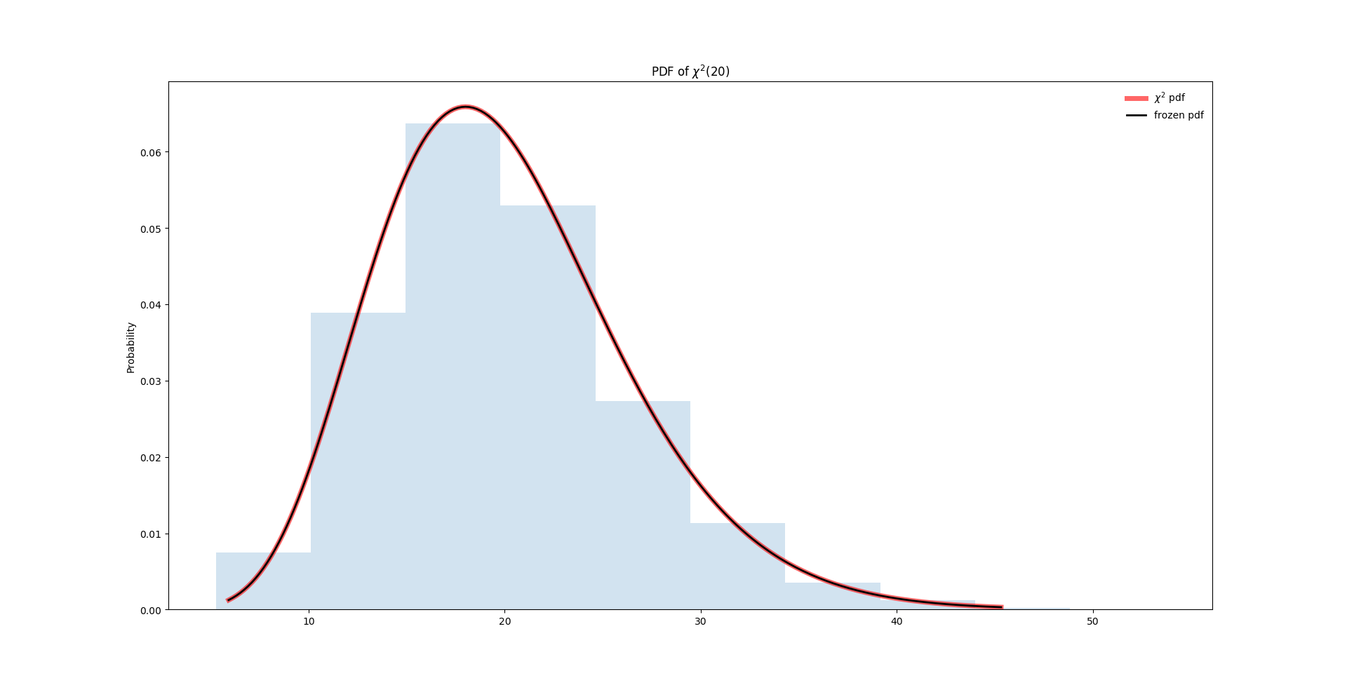
图2,卡方分布$\chi^2(20)$的PDF图
Python实现代码如下:
参考:https://docs.scipy.org/doc/scipy/reference/generated/scipy.stats.chi2.html#scipy.stats.chi2
 1 def chi2_distribution(df=1):
 2     """
 3     卡方分布,在实际的定义中只有一个参数df,即定义中的n
 4     :param df: 自由度,也就是该分布中独立变量的个数
 5     :return:
 6     """
 7
 8     fig, ax = plt.subplots(1, 1)
 9
10     # 直接传入参数, Display the probability density function (pdf)
11     x = np.linspace(stats.chi2.ppf(0.001, df),
12                     stats.chi2.ppf(0.999, df), 200)
13     ax.plot(x, stats.chi2.pdf(x, df), 'r-',
14             lw=5, alpha=0.6, label=r'$\chi^2$ pdf')
15
16     # 从冻结的均匀分布取值, Freeze the distribution and display the frozen pdf
17     chi2_dis = stats.chi2(df=df)
18     ax.plot(x, chi2_dis.pdf(x), 'k-',
19             lw=2, label='frozen pdf')
20
21     # 计算ppf分别等于0.001, 0.5, 0.999时的x值
22     vals = chi2_dis.ppf([0.001, 0.5, 0.999])
23     print(vals)  # [ 2.004  4.     5.996]
24
25     # Check accuracy of cdf and ppf
26     print(np.allclose([0.001, 0.5, 0.999], chi2_dis.cdf(vals)))  # Ture
27
28     # Generate random numbers
29     r = chi2_dis.rvs(size=10000)
30     ax.hist(r, normed=True, histtype='stepfilled', alpha=0.2)
31     plt.ylabel('Probability')
32     plt.title(r'PDF of $\chi^2$({})'.format(df))
33     ax.legend(loc='best', frameon=False)
34     plt.show()
35
36 chi2_distribution(df=20)
其实在scipy对卡方分布的说明中,卡方分布还有其他两个参数,loc和scale,默认情况下,$loc = 0$, $scale = 1$。这时相当于是一个标准化的卡方分布,可以根据loc和scale对函数进行平移和缩放。官方文档是这样描述的:
The probability density above is defined in the “standardized” form. To shift and/or scale the distribution use the loc and scale parameters. Specifically, chi2.pdf(x, df, loc, scale) is identically equivalent to chi2.pdf(y, df) / scale with y = (x - loc) / scale.
不同参数的卡方分布
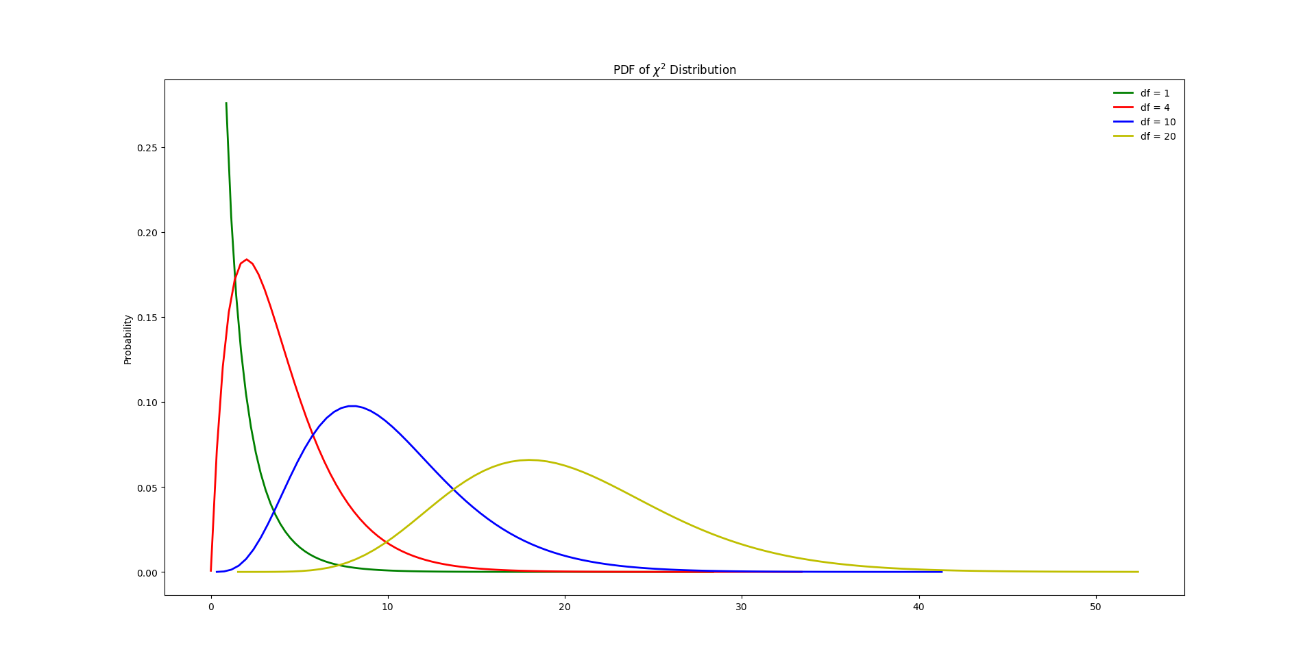
图3,不同参数下的卡方分布PDF图像
当自由度df等于1或2时,函数图像都呈单调递减的趋势;当df大于等于3时,呈先增后减的趋势。从定义上来看,df的值只能取正整数,但是实际上传入小数也可以做出图像(此时的df不知道该如何解释)。
图3的Python实现代码如下:
 1 def diff_chi2_dis():
 2     """
 3     不同参数下的卡方分布
 4     :return:
 5     """
 6     # chi2_dis_0_5 = stats.chi2(df=0.5)
 7     chi2_dis_1 = stats.chi2(df=1)
 8     chi2_dis_4 = stats.chi2(df=4)
 9     chi2_dis_10 = stats.chi2(df=10)
10     chi2_dis_20 = stats.chi2(df=20)
11
12     # x1 = np.linspace(chi2_dis_0_5.ppf(0.01), chi2_dis_0_5.ppf(0.99), 100)
13     x2 = np.linspace(chi2_dis_1.ppf(0.65), chi2_dis_1.ppf(0.9999999), 100)
14     x3 = np.linspace(chi2_dis_4.ppf(0.000001), chi2_dis_4.ppf(0.999999), 100)
15     x4 = np.linspace(chi2_dis_10.ppf(0.000001), chi2_dis_10.ppf(0.99999), 100)
16     x5 = np.linspace(chi2_dis_20.ppf(0.00000001), chi2_dis_20.ppf(0.9999), 100)
17     fig, ax = plt.subplots(1, 1)
18     # ax.plot(x1, chi2_dis_0_5.pdf(x1), 'b-', lw=2, label=r'df = 0.5')
19     ax.plot(x2, chi2_dis_1.pdf(x2), 'g-', lw=2, label='df = 1')
20     ax.plot(x3, chi2_dis_4.pdf(x3), 'r-', lw=2, label='df = 4')
21     ax.plot(x4, chi2_dis_10.pdf(x4), 'b-', lw=2, label='df = 10')
22     ax.plot(x5, chi2_dis_20.pdf(x5), 'y-', lw=2, label='df = 20')
23     plt.ylabel('Probability')
24     plt.title(r'PDF of $\chi^2$ Distribution')
25     ax.legend(loc='best', frameon=False)
26     plt.show()
27
28 diff_chi2_dis()
1.4 分位数的计算
第一种情况:给定上分位数$x_1$,求概率$P(X \geq x_1)$,这也是用的比较多的情况(在假设检验中计算P值)。按照上分位数的定义,如果要计算比$x_1$更大的取值的概率,只需要计算$1 - cdf(x_1)$就可以得到。
参考图2,我们分别计算在卡方分布$\chi^2(20)$中,$x = 20$以及$x = 40$时对应的$\alpha$值(或P值)。
>>> from scipy import stats
>>> 1 - stats.chi2.cdf(20, 20)
0.45792971447185216
>>> 1 - stats.chi2.cdf(40, 20)
0.0049954123083075785
上面的cdf函数有两个参数,第一个位置是$x$的值,第二个位置是$df$的值(degree of freedom,卡方分布的自由度)。从图2中也可以看到,$20$基本上位于卡方分布$\chi^2(20)$的PDF图像中间的位置,该位置右边基本上占了整个PDF的一半;$40$这个值非常靠右,该值右边的面积非常小,计算得出在该分布中只有大约0.5%的值大于40。
由于计算某个分布下特定$x$的$\alpha$值在统计的应用中非常重要,因此有专门的函数来做相关的计算,这个专门的函数在$\alpha$值非常小的情况下(即$x$的值在图像中非常靠右),计算出来的结果比上面的方法更精确。
下面是官方文档的说明:
Survival function (also defined as 1 - cdf, but sf is sometimes more accurate).
>>> stats.chi2.sf(20, 20)
0.45792971447185232
>>> stats.chi2.sf(40, 20)
0.0049954123083075785
>>> stats.chi2.sf(100, 20)
1.2596084591660847e-12
>>> 1 - stats.chi2.cdf(100, 20)
1.2596590437397026e-12
>>> 1 - stats.chi2.cdf(1000, 20)
0.0
>>> stats.chi2.sf(1000, 20)
3.9047966391213445e-199
从上面可以看到,当$x = 1000$时,用第一种方法的精度已经不够用了,但是第二种方法还是可以计算出一个非零的数值。
在介绍分位数时,说过在某个分布中,$x_{\alpha}$与$\alpha$知道其中一个,就可以计算出另一个值来。上面的方法是已知$x_{\alpha}$计算$\alpha$,下面是根据$\alpha$的值,求对应的$x_{\alpha}$,即上$\alpha$分位数。
>>> stats.chi2.isf(0.995, 20)
7.4338442629342243
>>> stats.chi2.isf(0.95, 20)
10.850811394182589
>>> stats.chi2.isf(0.5, 20)
19.337429229428256
>>> stats.chi2.isf(0.05, 20)
31.410432844230929
>>> stats.chi2.isf(0.005, 20)
39.996846312938651
看到0.05这样的值是不是很熟悉?其实这个过程就是我们学统计时查表的过程,通常概率论与数理统计方面的书后面的附表都会有常见分布的"上侧分位点表"。有了Python,我们以后就不需要翻书查表了。
参考这里:https://www.medcalc.org/manual/chi-square-table.php
这里的$\alpha$就相当于假设检验中的$p$值。
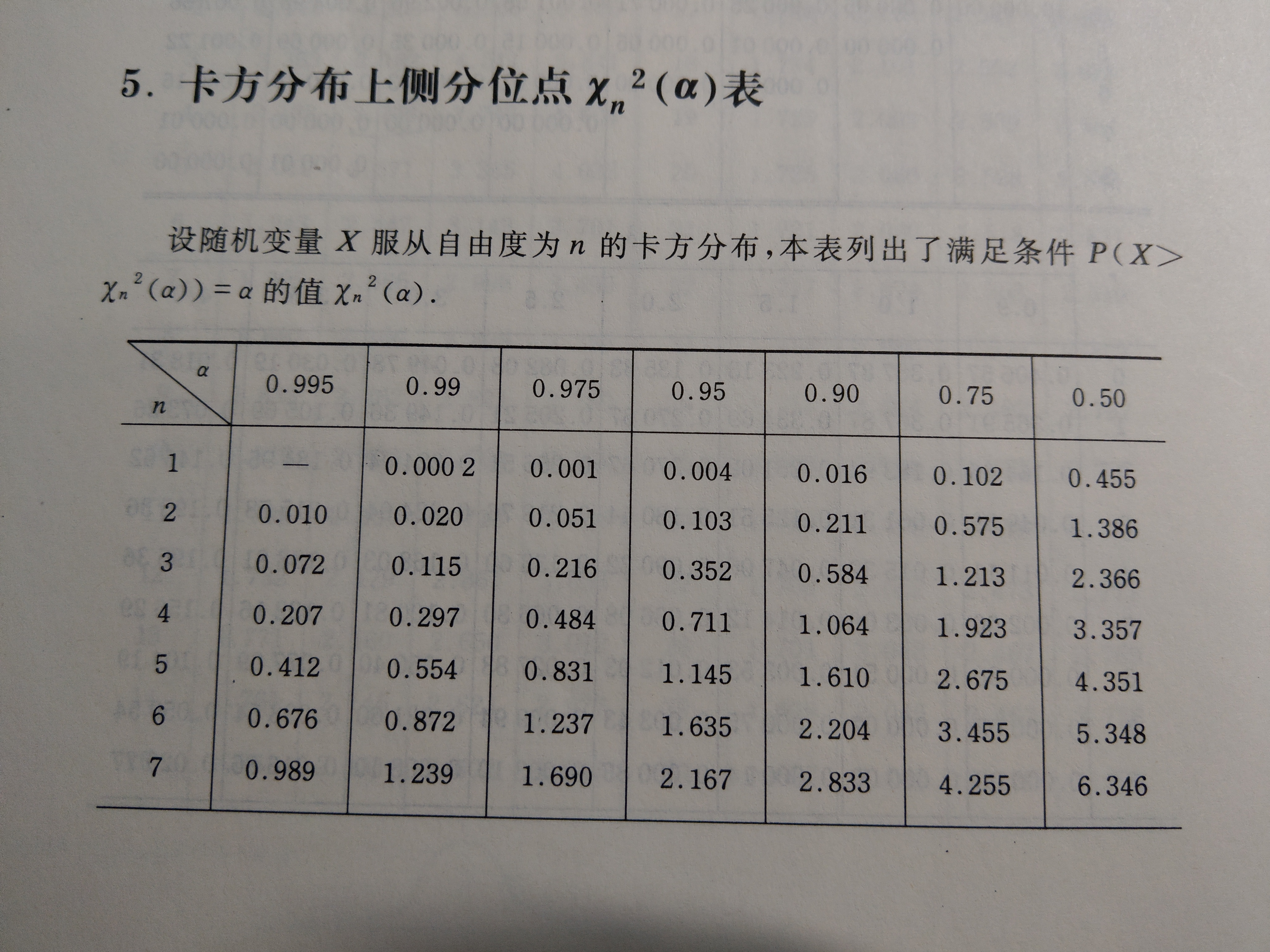
图4,统计相关书籍中的附表
2. t分布
t分布的推导最早由大地测量学家Friedrich Robert Helmert于1876年提出,并由数学家Lüroth证明。英国人威廉·戈塞(Willam S. Gosset)于1908年再次发现并发表了t分布,当时他还在爱尔兰都柏林的吉尼斯(Guinness)啤酒酿酒厂工作。酒厂虽然禁止员工发表一切与酿酒研究有关的成果,但允许他在不提到酿酒的前提下,以笔名发表t分布的发现,所以论文使用了“学生”(Student)这一笔名。之后t检验以及相关理论经由罗纳德·费雪(Sir Ronald Aylmer Fisher)发扬光大,为了感谢戈塞的功劳,费雪将此分布命名为学生t分布(Student's t)。
2.1 定义
设$X \sim N(0, 1), Y \sim \chi^2(n)$,且X和Y相互独立,则称随机变量$T = \frac{X} {\sqrt{Y/n}}$服从自由度为n的t分布,记为 $T \sim t(n)$。
- 当n=1的t分布,就是柯西分布
2.2 性质
设$T \sim t(n)$,则
- 当$n > 1$时,$E(T) = 0$,当$n = 1$时,期望不存在(参考柯西分布的期望,link)
- 当$n > 2$时,$D(T) = \frac{n} {n - 2}$,当$n \leq 2$时,方差不存在
2.3 函数图像
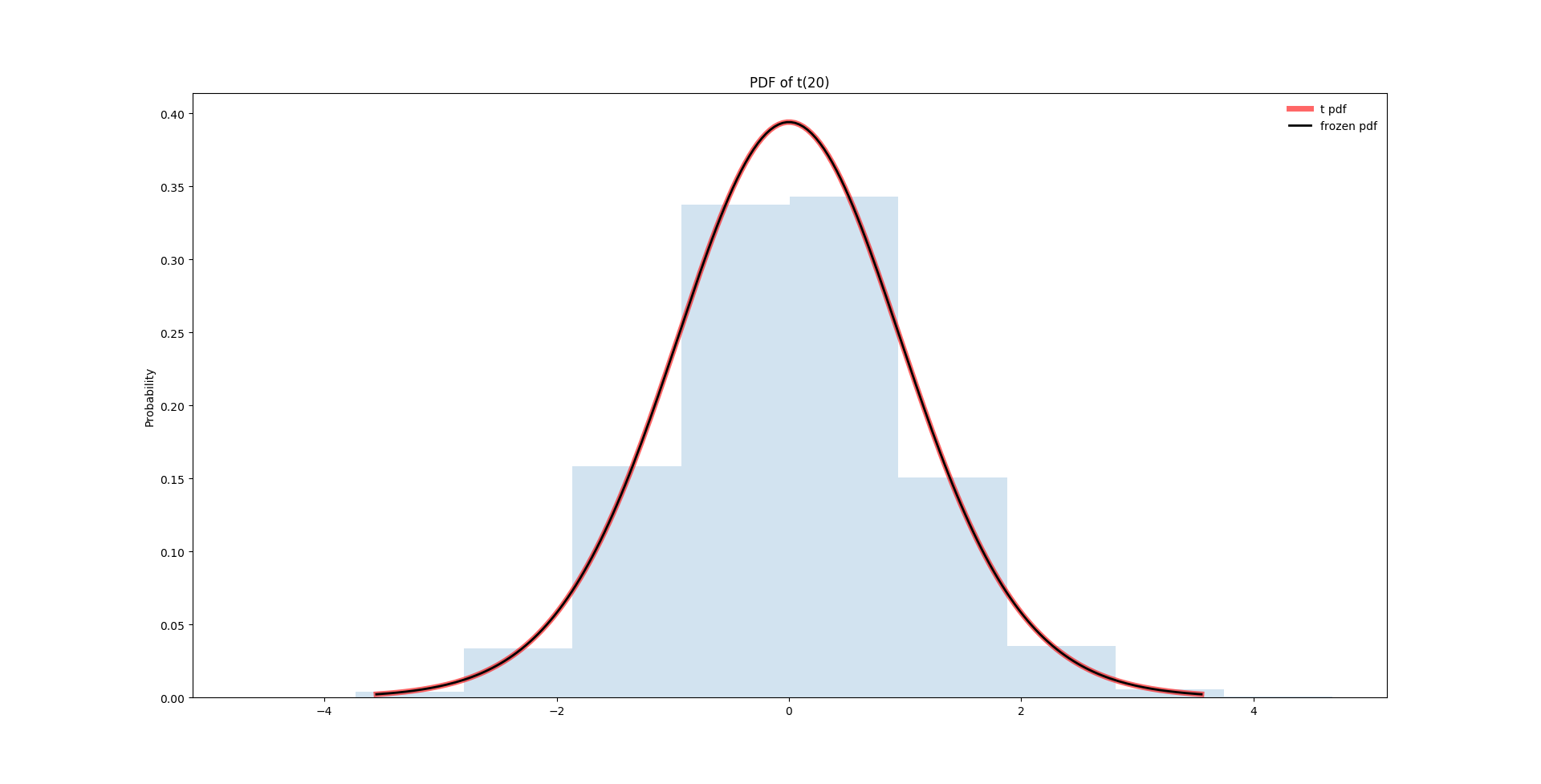
图5,t(20)的PDF图像
Python代码如下,更上面的代码差别不大:
参考:https://docs.scipy.org/doc/scipy/reference/generated/scipy.stats.t.html


 1 import numpy as np
 2 from scipy import stats
 3 import matplotlib.pyplot as plt
 4 # http://user.engineering.uiowa.edu/~dbricker/Stacks_pdf1/Sampling_Distns.pdf
 5 # https://docs.scipy.org/doc/scipy/reference/generated/scipy.stats.t.html
 6
 7
 8 def t_distribution(df=1.0):
 9     """
10     t分布,在实际的定义中只有一个参数df,即定义中的n
11     :param df: 自由度,也就是该分布包含的卡方分布中独立变量的个数
12     :return:
13     """
14
15     fig, ax = plt.subplots(1, 1)
16
17     # 直接传入参数, Display the probability density function (pdf)
18     x = np.linspace(stats.t.ppf(0.001, df),
19                     stats.t.ppf(0.999, df), 200)
20     ax.plot(x, stats.t.pdf(x, df), 'r-',
21             lw=5, alpha=0.6, label=r't pdf')
22
23     # 从冻结的t分布取值, Freeze the distribution and display the frozen pdf
24     t_dis = stats.t(df=df)
25     ax.plot(x, t_dis.pdf(x), 'k-',
26             lw=2, label='frozen pdf')
27
28     # 计算ppf分别等于0.001, 0.5, 0.999时的x值
29     vals = t_dis.ppf([0.001, 0.5, 0.999])
30     print(vals)  # [ -3.55180834e+00   6.72145055e-17   3.55180834e+00]
31
32     # Check accuracy of cdf and ppf
33     print(np.allclose([0.001, 0.5, 0.999], t_dis.cdf(vals)))  # Ture
34
35     # Generate random numbers
36     r = t_dis.rvs(size=10000)
37     ax.hist(r, normed=True, histtype='stepfilled', alpha=0.2)
38     plt.ylabel('Probability')
39     plt.title(r'PDF of t({})'.format(df))
40     ax.legend(loc='best', frameon=False)
41     plt.show()
42
43 t_distribution(df=20)
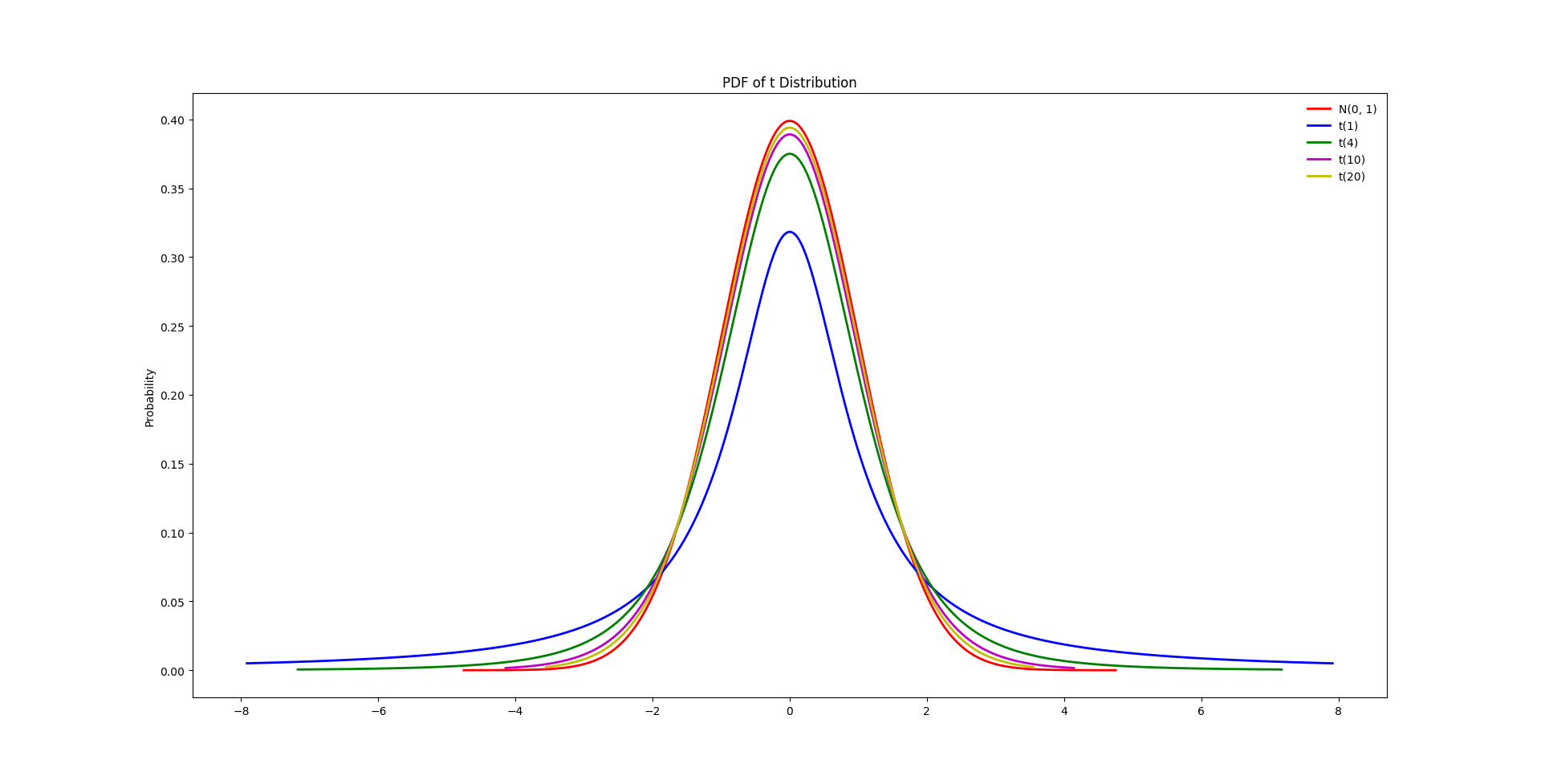
图6,不同参数下的t分布
从图6中可以看到,$t(1)$与标准正态分布之间的差别还是比较大的,但是当自由度n趋近于无穷大时,t分布与标准正态分布没有差别(公式上的形式将变得完全相同,这里没有列出概率密度函数的公式)。较大的区别在于,当自由度n较小时,t分布比标准正态分布的尾部更宽(fatter tails),因此也比正态分布更慢的趋近于0。关于这两类分布的异同将会在后面的假设检验部分详细阐述。
Python代码如下:
 1 def diff_t_dis():
 2     """
 3     不同参数下的t分布
 4     :return:
 5     """
 6     norm_dis = stats.norm()
 7     t_dis_1 = stats.t(df=1)
 8     t_dis_4 = stats.t(df=4)
 9     t_dis_10 = stats.t(df=10)
10     t_dis_20 = stats.t(df=20)
11
12     x1 = np.linspace(norm_dis.ppf(0.000001), norm_dis.ppf(0.999999), 1000)
13     x2 = np.linspace(t_dis_1.ppf(0.04), t_dis_1.ppf(0.96), 1000)
14     x3 = np.linspace(t_dis_4.ppf(0.001), t_dis_4.ppf(0.999), 1000)
15     x4 = np.linspace(t_dis_10.ppf(0.001), t_dis_10.ppf(0.999), 1000)
16     x5 = np.linspace(t_dis_20.ppf(0.001), t_dis_20.ppf(0.999), 1000)
17     fig, ax = plt.subplots(1, 1)
18     ax.plot(x1, norm_dis.pdf(x1), 'r-', lw=2, label=r'N(0, 1)')
19     ax.plot(x2, t_dis_1.pdf(x2), 'b-', lw=2, label='t(1)')
20     ax.plot(x3, t_dis_4.pdf(x3), 'g-', lw=2, label='t(4)')
21     ax.plot(x4, t_dis_10.pdf(x4), 'm-', lw=2, label='t(10)')
22     ax.plot(x5, t_dis_20.pdf(x5), 'y-', lw=2, label='t(20)')
23     plt.ylabel('Probability')
24     plt.title(r'PDF of t Distribution')
25     ax.legend(loc='best', frameon=False)
26     plt.show()
27
28 diff_t_dis()
2.4 t分布中上$\alpha$分位数的计算
在Python中的计算方法,参考1.4
3. F分布
F分布由两个卡方分布构成。
3.1 定义
设$X \sim \chi^2(n_1)$,$Y \sim \chi^2(n_2)$,且$X, Y$相互独立,则称随机变量$F = \frac{X/n_1} {Y/n_2}$服从自由度为$(n_1, n_2)$的F分布,记为$F \sim F(n_1, n_2)$。其中$n_1$称为第一自由度,$n_2$称为第二自由度。
3.2 性质
设$F \sim F(n, m)$,则
- $E(F) = \frac{m}{m - 2}$,其中$m \geq 2$,否则期望不存在
- $D(F) = \frac{2m^2(n + m - 2)} {n(m - 2)^2(m - 4)}$,其中$m \geq 4$,否则方差不存在
- $\frac{1} {F} \sim F(m, n)$,即F分布的倒数也是F分布(参数交换)
3.3 函数图像

图7,F(4, 10)的PDF图像
下面是Pyhon实现的代码,图7使用Spyder画出来的图,与上面使用Pycharm画出来的图差别还有点大。
参考:https://docs.scipy.org/doc/scipy/reference/generated/scipy.stats.f.html
 1 import numpy as np
 2 from scipy import stats
 3 import matplotlib.pyplot as plt
 4
 5
 6 def f_distribution(dfn=4, dfd=10):
 7     """
 8     F分布,有两个参数dfn, dfd,分别表示定义中的n1和n2
 9     :param dfn: 第一自由度,分子中卡方分布的自由度
10     :param dfd: 第二自由度,分母中卡方分布的自由度
11     :return:
12     """
13
14     fig, ax = plt.subplots(1, 1)
15
16     # 直接传入参数, Display the probability density function (pdf)
17     x = np.linspace(stats.f.ppf(0.0001, dfn, dfd),
18                     stats.f.ppf(0.999, dfn, dfd), 200)
19     ax.plot(x, stats.f.pdf(x, dfn, dfd), 'r-',
20             lw=5, alpha=0.6, label=r'f pdf')
21
22     # 从冻结的均匀分布取值, Freeze the distribution and display the frozen pdf
23     f_dis = stats.f(dfn=dfn, dfd=dfd)
24     ax.plot(x, f_dis.pdf(x), 'k-',
25             lw=2, label='frozen pdf')
26
27     # 计算ppf分别等于0.001, 0.5, 0.999时的x值
28     vals = f_dis.ppf([0.001, 0.5, 0.999])
29     print(vals)  # [  0.02081053   0.89881713  11.28275151]
30
31     # Check accuracy of cdf and ppf
32     print(np.allclose([0.001, 0.5, 0.999], f_dis.cdf(vals)))  # Ture
33
34     # Generate random numbers
35     r = f_dis.rvs(size=10000)
36     ax.hist(r, normed=True, histtype='stepfilled', alpha=0.2)
37     plt.ylabel('Probability')
38     plt.title(r'PDF of F({}, {})'.format(dfn, dfd))
39     ax.legend(loc='best', frameon=False)
40     plt.savefig('f_dist_pdf2.png', dip=200)
41
42 f_distribution(dfn=4, dfd=10)
F分布有两个参数,dfn和dfd,分别代表分子上的第一自由度和分母上的第二自由度。
下面是不同参数下,F分布的概率密度函数图像:
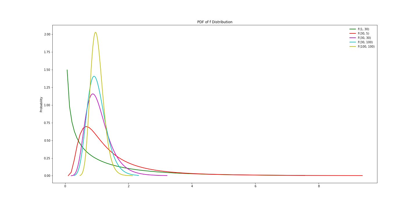
图8,不同参数下的F分布
Python实现的代码:
 1 def diff_f_dis():
 2     """
 3     不同参数下的F分布
 4     :return:
 5     """
 6 #    f_dis_0_5 = stats.f(dfn=10, dfd=1)
 7     f_dis_1_30 = stats.f(dfn=1, dfd=30)
 8     f_dis_30_5 = stats.f(dfn=30, dfd=5)
 9     f_dis_30_30 = stats.f(dfn=30, dfd=30)
10     f_dis_30_100 = stats.f(dfn=30, dfd=100)
11     f_dis_100_100 = stats.f(dfn=100, dfd=100)
12
13 #    x1 = np.linspace(f_dis_0_5.ppf(0.01), f_dis_0_5.ppf(0.99), 100)
14     x2 = np.linspace(f_dis_1_30.ppf(0.2), f_dis_1_30.ppf(0.99), 100)
15     x3 = np.linspace(f_dis_30_5.ppf(0.00001), f_dis_30_5.ppf(0.99), 100)
16     x4 = np.linspace(f_dis_30_30.ppf(0.00001), f_dis_30_30.ppf(0.999), 100)
17     x6 = np.linspace(f_dis_30_100.ppf(0.0001), f_dis_30_100.ppf(0.999), 100)
18     x5 = np.linspace(f_dis_100_100.ppf(0.0001), f_dis_100_100.ppf(0.9999), 100)
19     fig, ax = plt.subplots(1, 1, figsize=(20, 10))
20 #    ax.plot(x1, f_dis_0_5.pdf(x1), 'b-', lw=2, label=r'F(0.5, 0.5)')
21     ax.plot(x2, f_dis_1_30.pdf(x2), 'g-', lw=2, label='F(1, 30)')
22     ax.plot(x3, f_dis_30_5.pdf(x3), 'r-', lw=2, label='F(30, 5)')
23     ax.plot(x4, f_dis_30_30.pdf(x4), 'm-', lw=2, label='F(30, 30)')
24     ax.plot(x6, f_dis_30_100.pdf(x6), 'c-', lw=2, label='F(30, 100)')
25     ax.plot(x5, f_dis_100_100.pdf(x5), 'y-', lw=2, label='F(100, 100)')
26
27     plt.ylabel('Probability')
28     plt.title(r'PDF of f Distribution')
29     ax.legend(loc='best', frameon=False)
30     plt.savefig('f_diff_pdf.png', dip=500)
31     plt.show()
32
33 diff_f_dis()
3.4 分位数的计算
参考1.4
4. 三大抽样分布之间的联系
下面这个例子,可以展示这三大抽样分布于标准正态分布的联系,以及它们自身之间的联系:
$X, Y, Z$相互独立,且都服从$N(0, 1)$分布,那么:
- $X^2 + Y^2 + Z^2 \sim \chi^2(3)$
- $\frac{X} {\sqrt{(Y^2 + Z^2)/2}} \sim t(2)$
- $\frac{2X^2} {Y^2 + Z^2} \sim F(1, 2)$
- 若$t \sim t(n)$,那么$t^2 \sim F(1, n)$
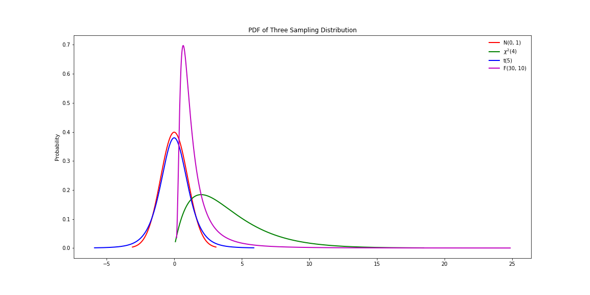
图9,三类抽样分布于标准正态分布之间的比较
从图9可以看到,t分布和标准正态分布都是左右对称的,偏度为0(偏度为0也可能不对称),但是卡方分布和F分布都不对称,呈正偏态(右侧的尾部更长,分布的主体集中在左侧)。
图9的Python代码如下:
 1 def three_sampling_dis():
 2     """
 3     三大抽样分布与标准正态分布
 4     :return:
 5     """
 6     nor_dis = stats.norm()
 7     chi2_dis = stats.chi2(df=4)
 8     t_dis = stats.t(df=5)
 9     f_dis = stats.f(dfn=30, dfd=5)
10
11     x1 = np.linspace(nor_dis.ppf(0.001), nor_dis.ppf(0.999), 1000)
12     x2 = np.linspace(chi2_dis.ppf(0.001), chi2_dis.ppf(0.999), 1000)
13     x3 = np.linspace(t_dis.ppf(0.001), t_dis.ppf(0.999), 1000)
14     x4 = np.linspace(f_dis.ppf(0.001), f_dis.ppf(0.999), 1000)
15     fig, ax = plt.subplots(1, 1, figsize=(16, 8))
16     ax.plot(x1, nor_dis.pdf(x1), 'r-', lw=2, label=r'N(0, 1)')
17     ax.plot(x2, chi2_dis.pdf(x2), 'g-', lw=2, label=r'$\chi^2$(4)')
18     ax.plot(x3, t_dis.pdf(x3), 'b-', lw=2, label='t(5)')
19     ax.plot(x4, f_dis.pdf(x4), 'm-', lw=2, label='F(30, 10)')
20
21     plt.ylabel('Probability')
22     plt.title(r'PDF of Three Sampling Distribution')
23     ax.legend(loc='best', frameon=False)
24     plt.savefig('diff_dist_pdf.png', dip=500)
25     plt.show()
26
27 three_sampling_dis()
欢迎阅读“概率论与数理统计及Python实现”系列文章
Reference
http://www.auburn.edu/~zengpen/teaching/table-chisq.pdf
https://en.wikipedia.org/wiki/F-distribution
http://mathworld.wolfram.com/F-Distribution.html
https://math.stackexchange.com/questions/1087106/find-the-mean-and-the-variance-of-an-f-random-variable-with-r-1-and-r-2-degr
https://zh.wikipedia.org/wiki/%E5%81%8F%E5%BA%A6
中国大学MOOC:浙江大学&哈工大,概率论与数理统计
修订记录:
9.14, 2020 补充说明上$\alpha$分位数的计算

 浙公网安备 33010602011771号