[Intro to Deep Learning with PyTorch -- L2 -- N9] Perceptron Trick

Give this:

 

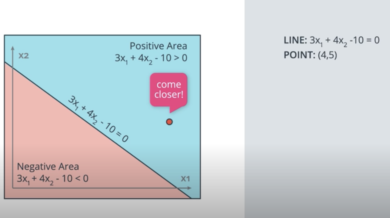
We have a wrongn classified point, how to move the line to come closer to the points?

We apply learning rate and since wrong point is in positive area, we need to  W - learning rate * wrong cord

 

The same, if the wrong point in negivate area, we do : W + learing rate * wrong cord:

 

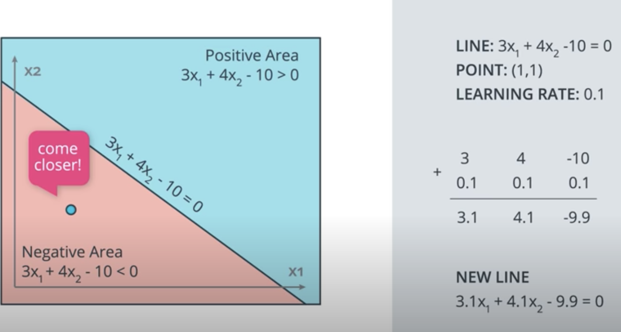
For the second example, where the line is described by 3x1+ 4x2 - 10 = 0, if the learning rate was set to 0.1, how many times would you have to apply the perceptron trick to move the line to a position where the blue point, at (1, 1), is correctly classified?

Answer: 10 times

 

Coding the Perceptron Algorithm

Time to code! In this quiz, you'll have the chance to implement the perceptron algorithm to separate the following data (given in the file data.csv).

Recall that the perceptron step works as follows. For a point with coordinates (p,q)(p,q), label yy, and prediction given by the equation \hat{y} = step(w_1x_1 + w_2x_2 + b)y^​=step(w1​x1​+w2​x2​+b):

• If the point is correctly classified, do nothing.
• If the point is classified positive, but it has a negative label, subtract \alpha p, \alpha q,αp,αq, and \alphaα from w_1, w_2,w1​,w2​, and bb respectively.
• If the point is classified negative, but it has a positive label, add \alpha p, \alpha q,αp,αq, and \alphaα to w_1, w_2,w1​,w2​, and bb respectively.

Then click on test run to graph the solution that the perceptron algorithm gives you. It'll actually draw a set of dotted lines, that show how the algorithm approaches to the best solution, given by the black solid line.

import numpy as np
# Setting the random seed, feel free to change it and see different solutions.
np.random.seed(42)

def stepFunction(t):
    if t >= 0:
        return 1
    return 0

def prediction(X, W, b):
    return stepFunction((np.matmul(X,W)+b)[0])

# TODO: Fill in the code below to implement the perceptron trick.
# The function should receive as inputs the data X, the labels y,
# the weights W (as an array), and the bias b,
# update the weights and bias W, b, according to the perceptron algorithm,
# and return W and b.
def perceptronStep(X, y, W, b, learn_rate = 0.01):
    for i in range(len(X)):
        y_hat = prediction(X[i], W, b)
        # predition in prostive area
        if y[i]-y_hat == -1:
            W[0] -= X[i][0]*learn_rate
            W[1] -= X[i][1]*learn_rate
            b -= learn_rate
        # predition in negivate area    
        elif y[i]-y_hat == 1:
            W[0] += X[i][0]*learn_rate
            W[1] += X[i][1]*learn_rate
            b += learn_rate
    
    return W, b
    
# This function runs the perceptron algorithm repeatedly on the dataset,
# and returns a few of the boundary lines obtained in the iterations,
# for plotting purposes.
# Feel free to play with the learning rate and the num_epochs,
# and see your results plotted below.
def trainPerceptronAlgorithm(X, y, learn_rate = 0.01, num_epochs = 25):
    x_min, x_max = min(X.T[0]), max(X.T[0])
    y_min, y_max = min(X.T[1]), max(X.T[1])
    W = np.array(np.random.rand(2,1))
    b = np.random.rand(1)[0] + x_max
    # These are the solution lines that get plotted below.
    boundary_lines = []
    for i in range(num_epochs):
        # In each epoch, we apply the perceptron step.
        W, b = perceptronStep(X, y, W, b, learn_rate)
        boundary_lines.append((-W[0]/W[1], -b/W[1]))
    return boundary_lines

0.78051,-0.063669,1
0.28774,0.29139,1
0.40714,0.17878,1
0.2923,0.4217,1
0.50922,0.35256,1
0.27785,0.10802,1
0.27527,0.33223,1
0.43999,0.31245,1
0.33557,0.42984,1
0.23448,0.24986,1
0.0084492,0.13658,1
0.12419,0.33595,1
0.25644,0.42624,1
0.4591,0.40426,1
0.44547,0.45117,1
0.42218,0.20118,1
0.49563,0.21445,1
0.30848,0.24306,1
0.39707,0.44438,1
0.32945,0.39217,1
0.40739,0.40271,1
0.3106,0.50702,1
0.49638,0.45384,1
0.10073,0.32053,1
0.69907,0.37307,1
0.29767,0.69648,1
0.15099,0.57341,1
0.16427,0.27759,1
0.33259,0.055964,1
0.53741,0.28637,1
0.19503,0.36879,1
0.40278,0.035148,1
0.21296,0.55169,1
0.48447,0.56991,1
0.25476,0.34596,1
0.21726,0.28641,1
0.67078,0.46538,1
0.3815,0.4622,1
0.53838,0.32774,1
0.4849,0.26071,1
0.37095,0.38809,1
0.54527,0.63911,1
0.32149,0.12007,1
0.42216,0.61666,1
0.10194,0.060408,1
0.15254,0.2168,1
0.45558,0.43769,1
0.28488,0.52142,1
0.27633,0.21264,1
0.39748,0.31902,1
0.5533,1,0
0.44274,0.59205,0
0.85176,0.6612,0
0.60436,0.86605,0
0.68243,0.48301,0
1,0.76815,0
0.72989,0.8107,0
0.67377,0.77975,0
0.78761,0.58177,0
0.71442,0.7668,0
0.49379,0.54226,0
0.78974,0.74233,0
0.67905,0.60921,0
0.6642,0.72519,0
0.79396,0.56789,0
0.70758,0.76022,0
0.59421,0.61857,0
0.49364,0.56224,0
0.77707,0.35025,0
0.79785,0.76921,0
0.70876,0.96764,0
0.69176,0.60865,0
0.66408,0.92075,0
0.65973,0.66666,0
0.64574,0.56845,0
0.89639,0.7085,0
0.85476,0.63167,0
0.62091,0.80424,0
0.79057,0.56108,0
0.58935,0.71582,0
0.56846,0.7406,0
0.65912,0.71548,0
0.70938,0.74041,0
0.59154,0.62927,0
0.45829,0.4641,0
0.79982,0.74847,0
0.60974,0.54757,0
0.68127,0.86985,0
0.76694,0.64736,0
0.69048,0.83058,0
0.68122,0.96541,0
0.73229,0.64245,0
0.76145,0.60138,0
0.58985,0.86955,0
0.73145,0.74516,0
0.77029,0.7014,0
0.73156,0.71782,0
0.44556,0.57991,0
0.85275,0.85987,0
0.51912,0.62359,0