无迹卡尔曼滤波-2

对于上一篇中的问题：X ∼ N(µ, σ^2 ) , Y = sin(X)要求随机变量Y的期望和方差。还有一种思路是对X进行采样，比如取500个采样点(这些采样点可以称为sigma点)，然后求取这些采样点的期望和方差。当采样值足够大时,结果与理论值接近。这种思路的问题显而易见，当随机变量维数增大时采样点的数量会急剧增加，比如一维需要500个采样点，二维就需要500^=250,000个采样点，三维情况下需要500^3=125,000,000个采样点，显然这样会造成严重的计算负担。无迹卡尔曼滤法中采用一种方法来选取2n+1个sigma点，n为随机变量维数。

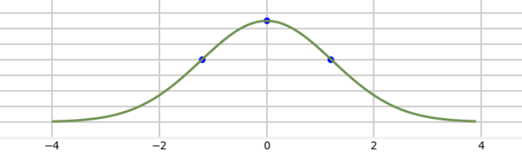
如上图所示，考虑正态分布曲线的对称性，选取3个sigma点来计算(sigma点的选取方法不唯一)，其中一个是均值，另外两个sigma点关于均值对称分布。比如三个点可选为：

χ₀ = μ;

χ₁ = μ + σ;

χ₂ = μ - σ;

然后选取合适的权值W_i满足如下关系_：

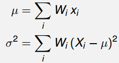
使用同样的公式近似计算Y=sin(X)分布的数字特征：

类比推广到多维随机变量X ∼ N(μ ,Σ)，Σ为协方差矩阵，采用Cholesky分解计算出矩阵L(Σ = LL^T)  ，矩阵L可以类比一维情况下的标准差σ。则sigma点可以写成下面的形式：

χ₀ = μ;

χ_i = μ + cL;

χ_n+i = μ - cL; c为一个正的常数

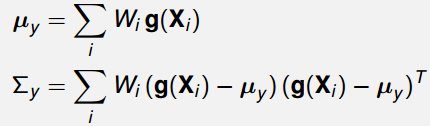
则对于非线性变换Y=g(X)，可以计算出变换后的期望和方差：

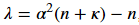
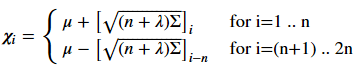
关键问题是如何选取sigma点和权值。常见的一种方法是第一个sigma点选为χ₀=μ，n是随机变量X的维数，α，κ，λ均为常数，并有如下关系

 

其余2n个sigma点的计算公式如下，其中下标i表示矩阵L的第i列

接下来要计算权值。对求期望来说，第一个sigma点的权值为：

对求方差来说，第一个sigma点的权值为如下，式子中的β也为一个常数

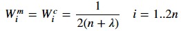
对于剩下的2n个sigma点来说求期望的权值和求方差的权值都相同：

因此，一共有三个常数(α,β,κ)需要我们来设定。根据其它参考资料，选择参数的经验为：β=2 is a good choice for Gaussian problems, κ=3−n is a good choice for κ , and 0≤α≤1 is an appropriate choice for α. 

α越大，第一个sigma点(平均值处)占的权重越大，并且其它sigma点越远离均值。如下图所示，对2维随机变量选取5个sigma点，点的大小代表权重，由感性认识可知sigma点离均值越远其权重应该越小。

 

根据上述计算步骤和公式我们可以编程实现sigma点的选择，权值的计算。在Python中我们可以采用现成的工具FilterPy安装pip工具后可以直接输入命令:pip install filterpy进行安装。

# -*- coding: utf-8 -*-
from filterpy.kalman import MerweScaledSigmaPoints as SigmaPoints

mean = 0    # 均值
cov =  1    # 方差

points = SigmaPoints(n=1, alpha=0.1, beta=2.0, kappa=1.0)  
Wm, Wc = points.weights()
sigmas = points.sigma_points(mean, cov)

print Wm, Wc    # 计算均值和方差的权值
print sigmas    # sigma点的坐标

对于标准正态分，输出结果如下:

 

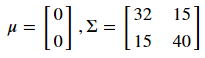
下面举一个2维正态分布的例子。从一个服从二维正态分布的随机变量中随机选取1000个点，该二维随机变量的期望和协方差矩阵为：

接下来将这1000个点进行如下非线性变换：

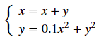
下面使用unscented transform方法近似计算非线性变换后随机变量的期望，并与直接从1000个点计算出的期望值对比

# -*- coding: utf-8 -*-
import numpy as np
from scipy import stats
import matplotlib.pyplot as plt
from numpy.random import multivariate_normal
from filterpy.kalman import unscented_transform
from filterpy.kalman import MerweScaledSigmaPoints as SigmaPoints

# 非线性变换函数
def f_nonlinear_xy(x, y):
    return np.array([x + y, 0.1*x**2 + y**2])

def plot1(xs, ys):
    xs = np.asarray(xs) 
    ys = np.asarray(ys)
    xmin = xs.min()
    xmax = xs.max()
    ymin = ys.min()
    ymax = ys.max()
    values = np.vstack([xs, ys])  
    kernel = stats.gaussian_kde(values)   
    X, Y = np.mgrid[xmin:xmax:100j, ymin:ymax:100j]
    positions = np.vstack([X.ravel(), Y.ravel()])
    Z = np.reshape(kernel.evaluate(positions).T, X.shape)  
    plt.imshow(np.rot90(Z),cmap=plt.cm.Greys,extent=[xmin, xmax, ymin, ymax])
    plt.plot(xs, ys, 'k.', markersize=2)
    plt.xlim(-20, 20)
    plt.ylim(-20, 20)
   
def plot2(xs, ys, f, mean_fx):
    fxs, fys = f(xs, ys)    # 将采样点进行非线性变换
    computed_mean_x = np.average(fxs)   
    computed_mean_y = np.average(fys)
    plt.subplot(121)
    plt.grid(False)
    plot1(xs, ys)
    plt.subplot(122)
    plt.grid(False)
    plot1(fxs, fys)
    plt.scatter(fxs, fys, marker='.', alpha=0.01, color='k')
    plt.scatter(mean_fx[0], mean_fx[1], marker='o', s=100, c='r', label='UT_mean')
    plt.scatter(computed_mean_x, computed_mean_y, marker='*',s=120, c='b', label='mean')
    plt.ylim([-10, 200])
    plt.xlim([-100, 100])
    plt.legend(loc='best', scatterpoints=1)
    print ('Difference in mean x={:.3f}, y={:.3f}'.format(
           computed_mean_x-mean_fx[0], computed_mean_y-mean_fx[1]))
    
# -------------------------------------------------------------------------------------------
mean = [0, 0]               # Mean of the N-dimensional distribution.
cov = [[32, 15], [15, 40]]  # Covariance matrix of the distribution.

# create sigma points(2n+1个sigma点)
# uses 3 parameters to control how the sigma points are distributed and weighted
points = SigmaPoints(n=2, alpha=.1, beta=2., kappa=1.)  
Wm, Wc = points.weights()
sigmas = points.sigma_points(mean, cov)

# pass through nonlinear function
sigmas_f = np.empty((5, 2))
for i in range(5):  
    sigmas_f[i] = f_nonlinear_xy(sigmas[i, 0], sigmas[i ,1]) 

# use unscented transform to get new mean and covariance
ukf_mean, ukf_cov = unscented_transform(sigmas_f, Wm, Wc)

# generate random points
xs, ys = multivariate_normal(mean, cov, size=1000).T  # 从二维随机变量的正态分布中产生1000个数据点
plot2(xs, ys, f_nonlinear_xy, ukf_mean)

# 画sigma点
plt.xlim(-30, 30); plt.ylim(0, 90)
plt.subplot(121)
plt.scatter(sigmas[:,0], sigmas[:,1], c='r', s=30) 
plt.show()

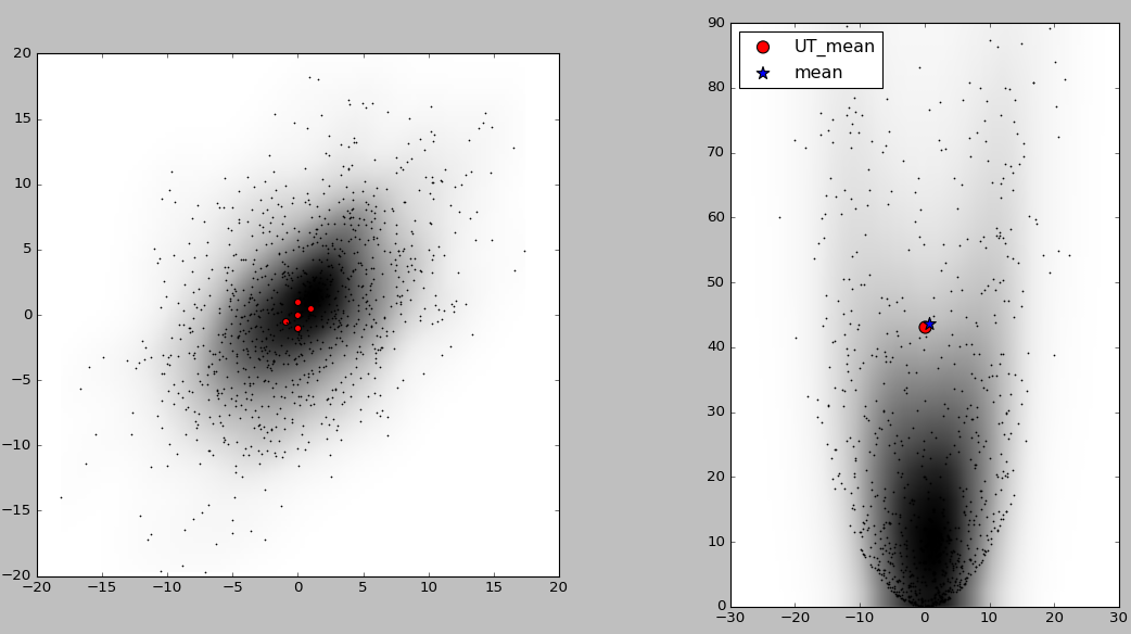
结果如下图所示，左图中黑点为1000个采样点，5个红色的点为sigma点，图中阴影表示概率密度的大小，颜色越深的地方概率密度越大。右图中的红点为用5个sigma点经UT变换计算出的近似期望，蓝色星号标记点为将1000个采样点非线性变换后直接计算出的期望。可以看出和直接产生1000个点经非线性变换计算期望相比,使用unscented transform的计算量要小的多，并且误差也不大。