实验二：逻辑回归算法实验

1导包和读取数据

#导包
import numpy as np
import pandas as pd
import matplotlib.pyplot as plt
#读取数据
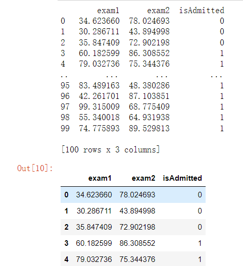
data=pd.read_csv("D:/1/ex2data1.txt",delimiter=',',header=None,names=['exam1','exam2','isAdmitted'])
print(data)
data.head()

 

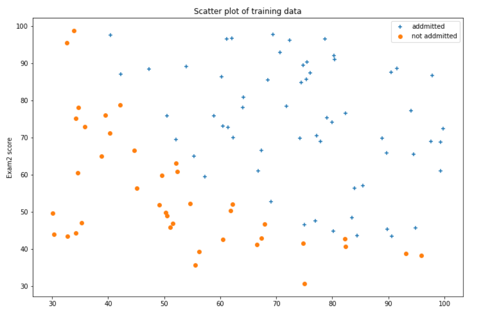
 2.绘制数据观察数据分布情况

admittedData=data[data['isAdmitted'].isin([1])]
noAdmittedData=data[data['isAdmitted'].isin([0])]
fig,ax=plt.subplots(figsize=(12,8))
ax.scatter(admittedData['exam1'],admittedData['exam2'],marker='+',label='addmitted')
ax.scatter(noAdmittedData['exam1'],noAdmittedData['exam2'],marker='o',label="not addmitted")
ax.legend(loc=1)
ax.set_xlabel('Exam1 score')
ax.set_ylabel('Exam2 score')
ax.set_title("Scatter plot of training data")
plt.show()

 

 

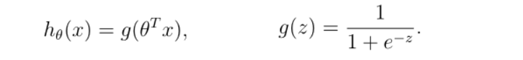
3编写sigmoid函数代码

def sigmoid(z):
return 1/(1+np.exp(-z))

 

 4编写逻辑回归代价函数代码

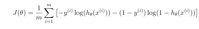
def computeCost(theta,X,Y):
theta = np.matrix(theta) 
h=sigmoid(np.dot(X,(theta.T)))
a=np.multiply(-Y,np.log(h))
b=np.multiply((1-Y),np.log(1-h))
return np.sum(a-b)/len(X)
computeCost(theta,X,Y) 

5编写梯度函数代码

 

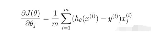
def gradient(theta,X,Y):
theta = np.matrix(theta) #要先把theta转化为矩阵
h = sigmoid(np.dot(X, (theta.T)))
grad = np.dot(((h-Y).T), X)/len(X)
return np.array(grad).flatten()

6编写寻找最优化参数代码

import scipy.optimize as opt
result = opt.fmin_tnc(func=computeCost, x0=theta, fprime=gradient, args=(X, Y))
print(result)
theta=result[0]

 

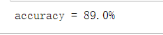
7 编写模型评估（预测）代码，输出预测准确率

def predict(theta, X):
theta = np.matrix(theta)
temp = sigmoid(X * theta.T)
#print(temp)
return [1 if x >= 0.5 else 0 for x in temp]
predictValues=predict(theta,X)
hypothesis=[1 if a==b else 0 for (a,b)in zip(predictValues,Y)]
accuracy=hypothesis.count(1)/len(hypothesis)
print ('accuracy = {0}%'.format(accuracy*100))

 

 

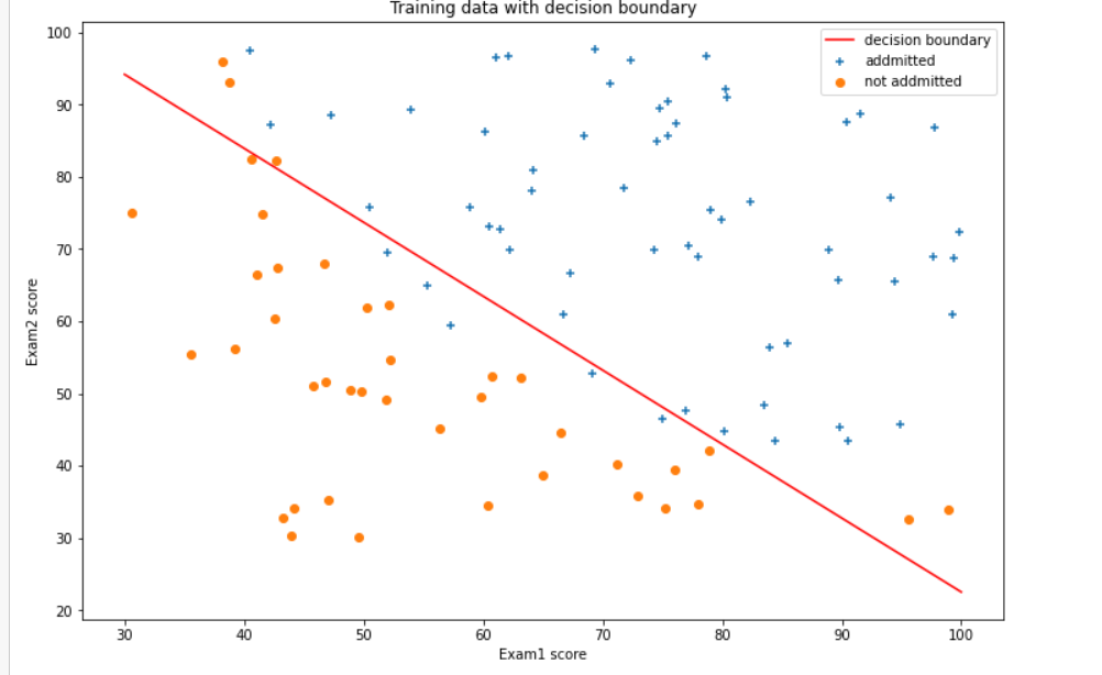
8寻找决策边界，画出决策边界直线图

#决策边界
def find_x2(x1,theta):
return [(-theta[0]-theta[1]*x_1)/theta[2] for x_1 in x1]
x1 = np.linspace(30, 100, 1000)
x2=find_x2(x1,theta)

admittedData=data[data['isAdmitted'].isin([1])]
noAdmittedData=data[data['isAdmitted'].isin([0])]
fig,ax=plt.subplots(figsize=(12,8))
ax.scatter(admittedData['exam1'],admittedData['exam2'],marker='+',label='addmitted')
ax.scatter(noAdmittedData['exam2'],noAdmittedData['exam1'],marker='o',label="not addmitted")
ax.plot(x1,x2,color='r',label="decision boundary")
ax.legend(loc=1)
ax.set_xlabel('Exam1 score')
ax.set_ylabel('Exam2 score')

ax.set_title("Training data with decision boundary")

plt.show()

 

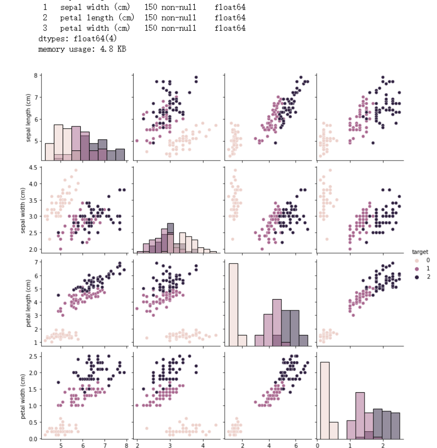
二. 针对iris数据集，应用sklearn库的逻辑回归算法进行类别预测。

1使用seaborn库进行数据可视化

 

import numpy as np
import pandas as pd
import matplotlib.pyplot as plt
import seaborn as sns
from sklearn.datasets import load_iris
data = load_iris()
iris_target = data.target
iris_features = pd.DataFrame(data=data.data, columns=data.feature_names)
iris_features.info()
iris_features.head()
iris_features.tail()
iris_target
pd.Series(iris_target).value_counts()
iris_features.describe()
iris_all = iris_features.copy()
iris_all['target'] = iris_target
sns.pairplot(data=iris_all,diag_kind='hist', hue= 'target')
plt.show()

 

 2将iri数据集分为训练集和测试集(两者比例为8:2)进行三分类训练和预测

from sklearn.model_selection import train_test_split
X_train,X_test,y_train,y_test = train_test_split(iris_features,iris_target,test_size=0.2,random_state=2020)
from sklearn.linear_model import LogisticRegression
clf=LogisticRegression(random_state=0,solver='lbfgs')
# 在训练集上训练逻辑回归模型
clf.fit(X_train,y_train)
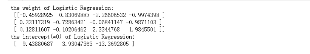
print('the weight of Logistic Regression:\n',clf.coef_)
print('the intercept(w0) of Logistic Regression:\n',clf.intercept_)
# 在训练集和测试集上分布进行预测
train_predict = clf.predict(x_train)
test_predict = clf.predict(x_test)

 

 3输出分类结果的混淆矩阵

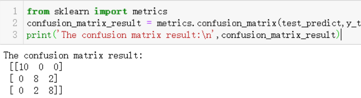
#查看混淆矩阵
confusion_matrix_result = metrics.confusion_matrix(test_predict,y_test)
print('混淆矩阵结果：\n',confusion_matrix_result)

 

 

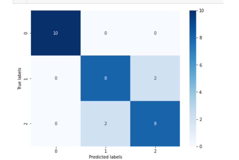
plt.figure(figsize=(8, 6))
sns.heatmap(confusion_matrix_result, annot=True, cmap='Blues')
plt.xlabel('Predicted labels')
plt.ylabel('True labels')
plt.show()