机器学习(Andrew Ng)作业代码(Exercise 1~2)

Programming Exercise 1: Linear Regression

单变量线性回归

warmUpExercise

要求：输出5阶单位阵
直接使用eye(5,5)即可

function A = warmUpExercise()
%WARMUPEXERCISE Example function in octave
%   A = WARMUPEXERCISE() is an example function that returns the 5x5 identity matrix

A = [];
% ============= YOUR CODE HERE ==============
% Instructions: Return the 5x5 identity matrix 
%               In octave, we return values by defining which variables
%               represent the return values (at the top of the file)
%               and then set them accordingly. 

A=eye(5,5);

% ===========================================
end

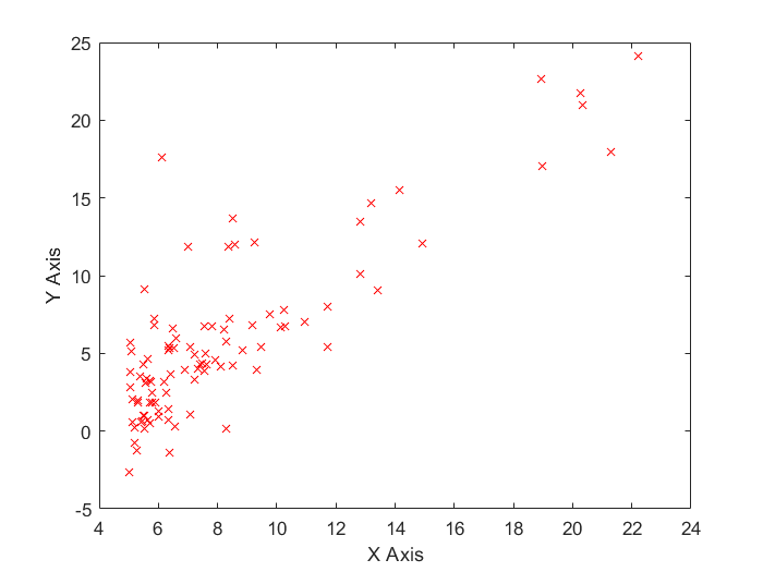
plotData

要求：读入若干组数据(x,y)，将它们绘制成散点图

使用MATLAB的plot()命令即可

function plotData(x, y)
%PLOTDATA Plots the data points x and y into a new figure 
%   PLOTDATA(x,y) plots the data points and gives the figure axes labels of
%   population and profit.

% ====================== YOUR CODE HERE ======================
% Instructions: Plot the training data into a figure using the 
%               "figure" and "plot" commands. Set the axes labels using
%               the "xlabel" and "ylabel" commands. Assume the 
%               population and revenue data have been passed in
%               as the x and y arguments of this function.
%
% Hint: You can use the 'rx' option with plot to have the markers
%       appear as red crosses. Furthermore, you can make the
%       markers larger by using plot(..., 'rx', 'MarkerSize', 10);

    figure; % open a new figure window

    data=load('ex1data1.txt');
    [n,m]=size(data);
    xdata=data(:,1);
    ydata=data(:,2);
    for i=1:n
        plot(xdata,ydata,'rx');
    end
    xlabel('X Axis');
    ylabel('Y Axis');
% ============================================================
end

输出结果：

computeCost

要求：读入\(m\)组数据(X,y)，计算用\(y=\theta^T X(\theta=(\theta_0,\theta_1)^T,X=(1,x^{(i)})^T)\)拟合这组数据的均方误差\(J(\theta)\)

\[J(\theta)=\frac 1 {2m}\sum_{i=1}^m(\theta^T X^{(i)}-y^{(i)})^2 \]

function J = computeCost(X, y, theta)
%传入:X为m*2矩阵，每一行第一列为1，第二个为X值,y为m维行向量，theta为二维列向量
%COMPUTECOST Compute cost for linear regression
%   J = COMPUTECOST(X, y, theta) computes the cost of using theta as the
%   parameter for linear regression to fit the data points in X and y

% Initialize some useful values
    m = length(y); % number of training examples

% You need to return the following variables correctly 
    J = 0;

% ====================== YOUR CODE HERE ======================
% Instructions: Compute the cost of a particular choice of theta
%               You should set J to the cost.

    for i=1:m
        J=J+(theta'*X(i,:)'-y(i))^2;
    end

    J=J/(2*m);

% =========================================================================
end

gradientDescent

要求：给出m组数据\((x^{(i)},y^{(i)})\)，学习率\(\alpha\)，梯度下降法迭代num_iters次后返回最终的参数\(\theta\)和每次迭代后的均方误差损失J_history

公式推导：

\[J(\theta)=\frac 1 {2m}\sum_{i=1}^m(\theta_0 +\theta_1 x^{(i)}-y^{(i)})^2 \]

\[\frac{\partial J(\theta)}{\partial \theta_0}= \frac 1 m \sum_{i=1}^m(\theta_0 +\theta_1 x^{(i)}-y^{(i)}) \]

\[\frac{\partial J(\theta)}{\partial \theta_1}= \frac 1 m \sum_{i=1}^m(\theta_0 +\theta_1 x^{(i)}-y^{(i)})x^{(i)} \]

梯度下降过程中，每次迭代同时更新\(\theta_0,\theta_1\)：

\[\theta _0 := \theta _0- \alpha \frac{\partial J(\theta)}{\partial \theta_0} \]

\[\theta _1 := \theta _1- \alpha \frac{\partial J(\theta)}{\partial \theta_1} \]

function [theta, J_history] = gradientDescent(X, y, theta, alpha, num_iters)
%GRADIENTDESCENT Performs gradient descent to learn theta
%   theta = GRADIENTDESENT(X, y, theta, alpha, num_iters) updates theta by 
%   taking num_iters gradient steps with learning rate alpha

% Initialize some useful values
m = length(y); % number of training examples
J_history = zeros(num_iters, 1);

for iter = 1:num_iters

    % ====================== YOUR CODE HERE ======================
    % Instructions: Perform a single gradient step on the parameter vector
    %               theta. 
    %
    % Hint: While debugging, it can be useful to print out the values
    %       of the cost function (computeCost) and gradient here.
    %

    dJ_dtheta0=0;
    dJ_dtheta1=0;
    for i=1:m
        dJ_dtheta0=dJ_dtheta0+(theta'*X(i,:)'-y(i));
        dJ_dtheta1=dJ_dtheta1+(theta'*X(i,:)'-y(i))*X(i,2);
    end
    dJ_dtheta0=dJ_dtheta0/m;
    dJ_dtheta1=dJ_dtheta1/m;
    theta=theta-alpha*([dJ_dtheta0,dJ_dtheta1])';
    % ============================================================

    % Save the cost J in every iteration    
    J_history(iter) = computeCost(X, y, theta)

end

end

最终运行结果

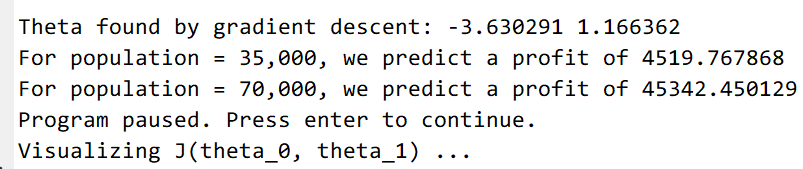
Fig1.梯度下降法线性回归拟合出的直线

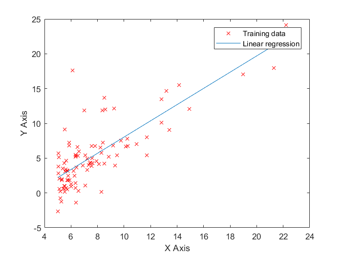
Fig2.\(J(\theta)\)的曲面图像

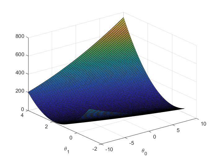
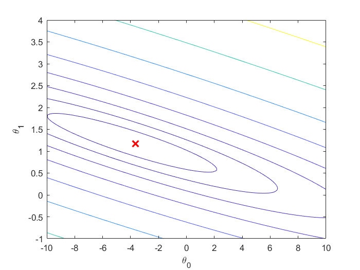
Fig3.\(J(\theta)\)的等高线图，红叉代表了\(J(\theta)\)最小处的点

多变量线性回归

featureNormalize

要求：给出m组输入数据的特征(这里特征维数为2)，即m行2列矩阵X，将输入数据Z-score归一化到区间[-1,1]。注意，这时还没有给X添加一列1

Z-score归一化方法：
对于第i维特征，计算出m组数据该特征的平均值\(\mu\)和标准差\(\sigma\)，则

\[x_i^{(t)}:=\frac {x_i^{(t)}-\mu}{\sigma} \]

归一化后每一维特征平均值为0，标准差为1

function [X_norm, mu, sigma] = featureNormalize(X)
%FEATURENORMALIZE Normalizes the features in X 
%   FEATURENORMALIZE(X) returns a normalized version of X where
%   the mean value of each feature is 0 and the standard deviation
%   is 1. This is often a good preprocessing step to do when
%   working with learning algorithms.

% You need to set these values correctly
X_norm = X;
mu = zeros(1, size(X, 2));
sigma = zeros(1, size(X, 2));

% ====================== YOUR CODE HERE ======================
% Instructions: First, for each feature dimension, compute the mean
%               of the feature and subtract it from the dataset,
%               storing the mean value in mu. Next, compute the 
%               standard deviation of each feature and divide
%               each feature by it's standard deviation, storing
%               the standard deviation in sigma. 
%
%               Note that X is a matrix where each column is a 
%               feature and each row is an example. You need 
%               to perform the normalization separately for 
%               each feature. 
%
% Hint: You might find the 'mean' and 'std' functions useful.
%       

    mu(1,1)=mean(X(:,1));
    mu(1,2)=mean(X(:,2));
    sigma(1,1)=std(X(:,1));
    sigma(1,2)=std(X(:,2));
    X_norm(:,1)=(X_norm(:,1)-mu(1,1))/sigma(1,1);
    X_norm(:,2)=(X_norm(:,2)-mu(1,2))/sigma(1,2);
% ============================================================

end

computeCostMulti

要求：给出m组输入数据(m*3矩阵X，每一行第一列为1)和真实输出y，计算用\(y=\theta^TX^{(i)T}\)拟合这些数据的均方误差\(J(\theta)\)

\[J(\theta)=\frac 1 {2m}\sum_{i=1}^m(\theta^TX^{(i)T}-y^{(i)})^2 \]

function J = computeCostMulti(X, y, theta)
%COMPUTECOSTMULTI Compute cost for linear regression with multiple variables
%   J = COMPUTECOSTMULTI(X, y, theta) computes the cost of using theta as the
%   parameter for linear regression to fit the data points in X and y

% Initialize some useful values
m = length(y); % number of training examples

% You need to return the following variables correctly 
J = 0;

% ====================== YOUR CODE HERE ======================
% Instructions: Compute the cost of a particular choice of theta
%               You should set J to the cost.
    for i=1:m
        J=J+(theta'*X(i)'-y(i))^2;
    end
    J=J/(2*m);
% =========================================================================

end

gradientDescentMulti

要求：给出m组数据\((x^{(i)},y^{(i)})\)，学习率\(\alpha\)，梯度下降法迭代num_iters次后返回最终的参数\(\theta\)和每次迭代后的均方误差损失J_history

注意，这里每个输入数据的第一维特征都是1(后来补上的)

公式推导：
对于第t个参数\(\theta_t\)，其更新公式为：

\[\theta _t := \theta _t- \alpha \frac{\partial J(\theta)}{\partial \theta_t} \]

\[\frac{\partial J(\theta)}{\partial \theta_t}= \frac 1 m \sum_{i=1}^m(\theta^TX^{(i)T}-y^{(i)})x_t^{(i)}\]

function [theta, J_history] = gradientDescentMulti(X, y, theta, alpha, num_iters)
%GRADIENTDESCENTMULTI Performs gradient descent to learn theta
%   theta = GRADIENTDESCENTMULTI(x, y, theta, alpha, num_iters) updates theta by
%   taking num_iters gradient steps with learning rate alpha

% Initialize some useful values
m = length(y); % number of training examples
J_history = zeros(num_iters, 1);

for iter = 1:num_iters

    % ====================== YOUR CODE HERE ======================
    % Instructions: Perform a single gradient step on the parameter vector
    %               theta. 
    %
    % Hint: While debugging, it can be useful to print out the values
    %       of the cost function (computeCostMulti) and gradient here.
    %
    paramsize=length(theta);
    dJ_dtheta=zeros(paramsize,1);
    for i=1:paramsize
        for j=1:m
            dJ_dtheta(i,1)=dJ_dtheta(i,1)+(theta'*X(j,:)'-y(j))*X(j,i);
        end
    end
    for i=1:paramsize
        dJ_dtheta(i,1)=dJ_dtheta(i,1)/m;
        theta(i)=theta(i)-alpha*dJ_dtheta(i);
    end
    % ============================================================

    % Save the cost J in every iteration    
    J_history(iter) = computeCostMulti(X, y, theta);

end

end

最终测试结果

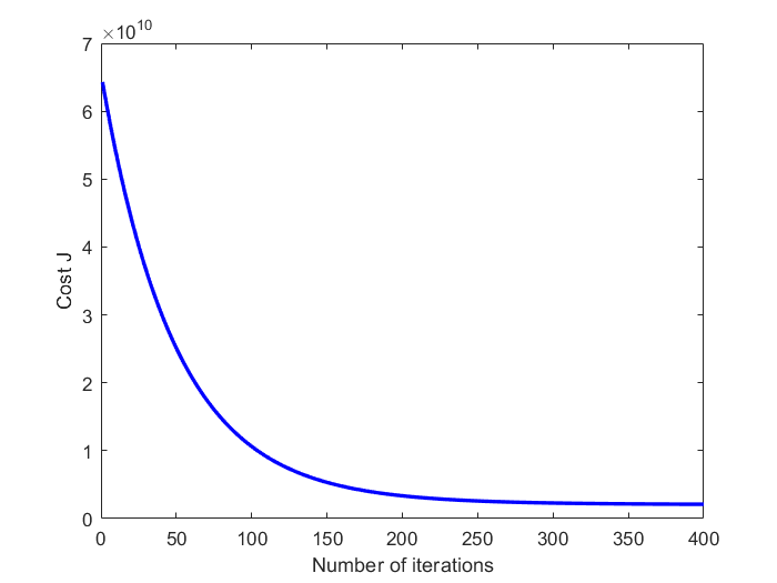
Fig1.收敛曲线

最小二乘法(投影法)求\(\theta\)

对于单变量的线性回归问题，

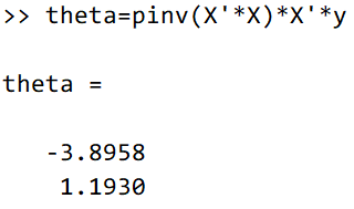
结果与梯度下降法近似。

Programming Exercise 2: Logistic Regression

Logistic回归二分类

plotData

function plotData(X, y)
%PLOTDATA Plots the data points X and y into a new figure 
%   PLOTDATA(x,y) plots the data points with + for the positive examples
%   and o for the negative examples. X is assumed to be a Mx2 matrix.

% Create New Figure
figure; hold on;

% ====================== YOUR CODE HERE ======================
% Instructions: Plot the positive and negative examples on a
%               2D plot, using the option 'k+' for the positive
%               examples and 'ko' for the negative examples.
%

    m=size(X,1);

    pos=find(y==1);
    neg=find(y==0);

    plot(X(pos,1),X(pos,2),'+','LineWidth', 2,'MarkerSize', 7);
    plot(X(neg,1),X(neg,2),'o', 'MarkerFaceColor', 'y','MarkerSize', 7);
% =========================================================================



hold off;

end

sigmoid

Sigmoid函数：

\[Sigmoid(x)=\frac 1 {1+e^{-x}} \]

function g = sigmoid(z)
%SIGMOID Compute sigmoid functoon
%   J = SIGMOID(z) computes the sigmoid of z.

% You need to return the following variables correctly 
g = zeros(size(z));

% ====================== YOUR CODE HERE ======================
% Instructions: Compute the sigmoid of each value of z (z can be a matrix,
%               vector or scalar).

    g=1/(1+exp(-z));

% =============================================================

end

costFunction

Logistic回归采用交叉熵误差函数：

\[J(\theta)=\frac 1 m \sum_{i=1}^m[-y^{(i)}log(h_\theta(X^{(i)}))-(1-y^{(i)})log(1-h_\theta(X^{(i)}))] \]

梯度下降公式推导：

\[Sigmoid'(x)=Sigmoid(x)(1-Sigmoid(x)) \]

\[\frac{\partial J(\theta)}{\partial \theta_t}=\frac 1 m \sum_{i=1}^m\ [-y^{(i)}\frac {g(\theta^T X^{(i)})(1-g(\theta^T X^{(i)}))}{{h_\theta(X^{(i)})}}-(1-y^{(i)})\frac {-g(\theta^T X^{(i)})(1-g(\theta^T X^{(i)}))}{1-h_\theta (X^{(i)})}]x_t^{(i)} \]

\[=\frac 1 m \sum_{i=1}^m\ [-y^{(i)}(1-g(\theta^T X^{(i)}))+(1-y^{(i)})g(\theta^T X^{(i)})]x_t^{(i)} \]

\[=\frac 1 m \sum_{i=1}^m\ (g(\theta^T X^{(i)})-y^{(i)})x_t^{(i)} \]

function [J, grad] = costFunction(theta, X, y)
%COSTFUNCTION Compute cost and gradient for logistic regression
%   J = COSTFUNCTION(theta, X, y) computes the cost of using theta as the
%   parameter for logistic regression and the gradient of the cost
%   w.r.t. to the parameters.

% Initialize some useful values
m = length(y); % number of training examples

% You need to return the following variables correctly 
J = 0;
grad = zeros(size(theta));

% ====================== YOUR CODE HERE ======================
% Instructions: Compute the cost of a particular choice of theta.
%               You should set J to the cost.
%               Compute the partial derivatives and set grad to the partial
%               derivatives of the cost w.r.t. each parameter in theta
%
% Note: grad should have the same dimensions as theta
%

    for i=1:m
        J=J+(-y(i)*log(sigmoid(theta'*X(i,:)'))-(1-y(i))*log(1-sigmoid(theta'*X(i,:)')));
    end
    
    J=J/m;
    
    for t=1:size(theta)
        for i=1:m
            grad(t)=grad(t)+(sigmoid(theta'*X(i,:)')-y(i))*X(i,t);
        end
        grad(t)=grad(t)/m;
    end

% =============================================================

end

predict

function p = predict(theta, X)
%PREDICT Predict whether the label is 0 or 1 using learned logistic 
%regression parameters theta
%   p = PREDICT(theta, X) computes the predictions for X using a 
%   threshold at 0.5 (i.e., if sigmoid(theta'*x) >= 0.5, predict 1)

m = size(X, 1); % Number of training examples

% You need to return the following variables correctly
p = zeros(m, 1);

% ====================== YOUR CODE HERE ======================
% Instructions: Complete the following code to make predictions using
%               your learned logistic regression parameters. 
%               You should set p to a vector of 0's and 1's
%

    for i=1:m
        tmp=theta'*X(i,:)';
        if(tmp>=0)
            p(i)=1;
        else
            p(i)=0;
        end
    end
% =========================================================================


end

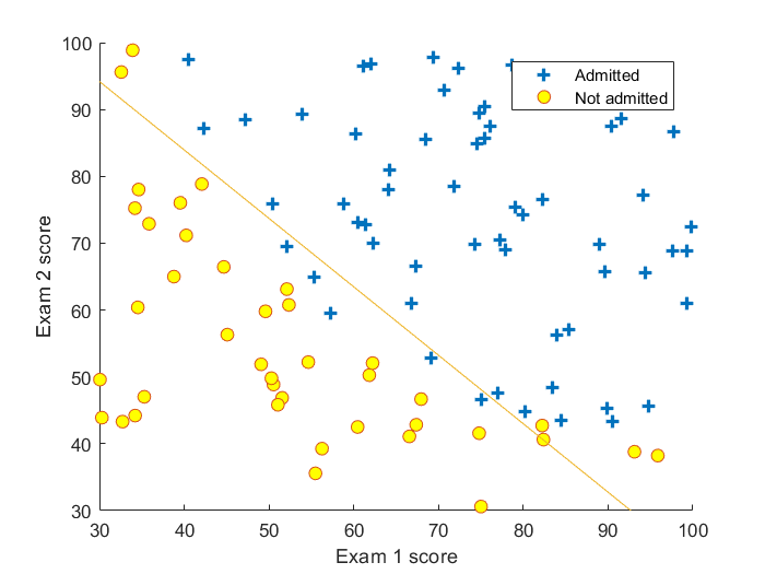
最终测试结果

带正则化的Logistic回归二分类

costFunctionReg

带正则化的Logistic回归中，损失函数加入了正则化项

\[J(\theta)=\frac 1 m \sum_{i=1}^m[-y^{(i)}log(h_\theta(X^{(i)}))-(1-y^{(i)})log(1-h_\theta(X^{(i)}))]+\frac \lambda {2m} \sum_{i=1}^n \theta_i^2 \]

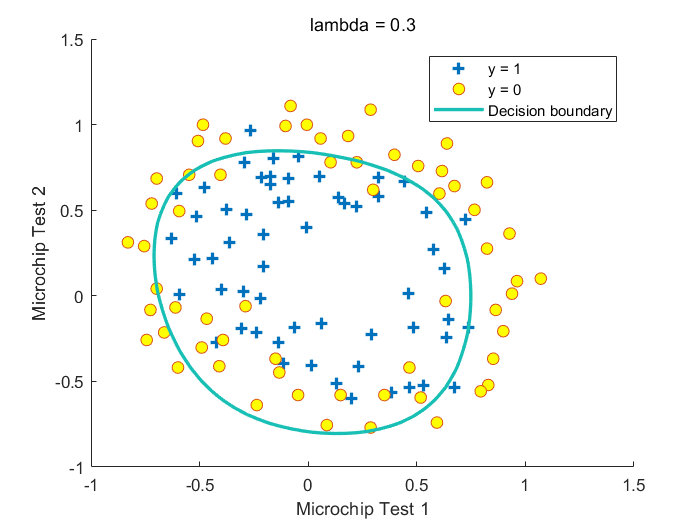
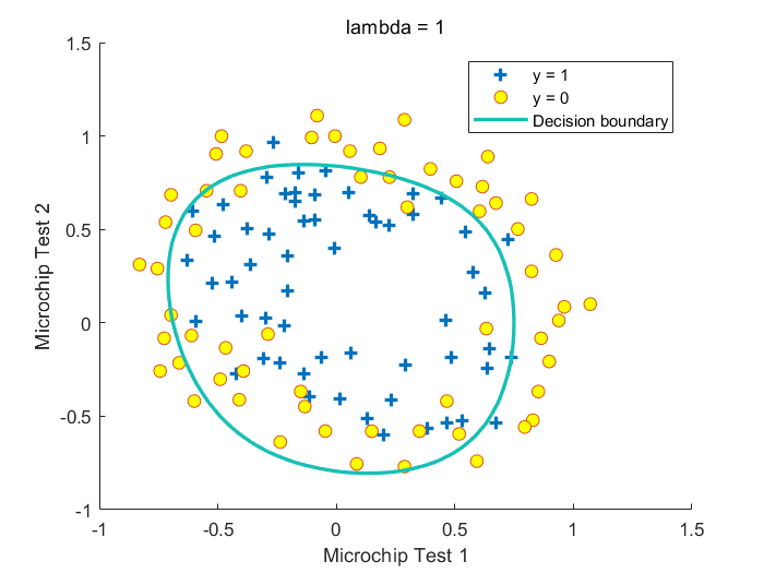
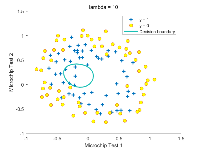
其中\(\lambda\)为惩罚参数，\(\lambda\)越大，\(\theta_1\cdots \theta_n\)越小，\(h_\theta(X)\)越接近\(Sigmoid(\theta_0)\)，越不容易过拟合，倾向于欠拟合。注意这里没有把\(\theta_0\)加入正则化项中

梯度下降公式推导：

\[Sigmoid'(x)=Sigmoid(x)(1-Sigmoid(x)) \]

\[\frac{\partial J(\theta)}{\partial \theta_0}=\frac 1 m \sum_{i=1}^m\ [-y^{(i)}\frac {g(\theta^T X^{(i)})(1-g(\theta^T X^{(i)}))}{{h_\theta(X^{(i)})}}-(1-y^{(i)})\frac {-g(\theta^T X^{(i)})(1-g(\theta^T X^{(i)}))}{1-h_\theta (X^{(i)})}]x_0^{(i)} \]

\[=\frac 1 m \sum_{i=1}^m\ [-y^{(i)}(1-g(\theta^T X^{(i)}))+(1-y^{(i)})g(\theta^T X^{(i)})]x_0^{(i)} \]

\[=\frac 1 m \sum_{i=1}^m\ (g(\theta^T X^{(i)})-y^{(i)})x_0^{(i)} \]

\[\frac{\partial J(\theta)}{\partial \theta_t}=\frac 1 m \sum_{i=1}^m\ [-y^{(i)}\frac {g(\theta^T X^{(i)})(1-g(\theta^T X^{(i)}))}{{h_\theta(X^{(i)})}}-(1-y^{(i)})\frac {-g(\theta^T X^{(i)})(1-g(\theta^T X^{(i)}))}{1-h_\theta (X^{(i)})}]x_t^{(i)}+\frac \lambda m \theta_t \]

\[=\frac 1 m \sum_{i=1}^m\ [-y^{(i)}(1-g(\theta^T X^{(i)}))+(1-y^{(i)})g(\theta^T X^{(i)})]x_t^{(i)}+\frac \lambda m \theta_t \]

\[=\frac 1 m \sum_{i=1}^m\ (g(\theta^T X^{(i)})-y^{(i)})x_t^{(i)}+\frac \lambda m \theta_t,\ \ \ \ t> 1 \]

function [J, grad] = costFunctionReg(theta, X, y, lambda)
%COSTFUNCTIONREG Compute cost and gradient for logistic regression with regularization
%   J = COSTFUNCTIONREG(theta, X, y, lambda) computes the cost of using
%   theta as the parameter for regularized logistic regression and the
%   gradient of the cost w.r.t. to the parameters. 

% Initialize some useful values
m = length(y); % number of training examples

% You need to return the following variables correctly 
J = 0;
grad = zeros(size(theta));

% ====================== YOUR CODE HERE ======================
% Instructions: Compute the cost of a particular choice of theta.
%               You should set J to the cost.
%               Compute the partial derivatives and set grad to the partial
%               derivatives of the cost w.r.t. each parameter in theta

    for i=1:m
        tmp=sigmoid(theta'*X(i,:)');
        J=J+(-y(i)*log(tmp)-(1-y(i))*log(1-tmp));
    end
    J=J/m;
    
    regsum=0;
    for i=2:size(theta)
        regsum=regsum+theta(i)*theta(i);
    end
    
    regsum=regsum*lambda/(2*m);
    
    J=J+regsum;

    for i=1:m
        grad(1)=grad(1)+(sigmoid(theta'*X(i,:)')-y(i))*X(i,1);
    end
    
    grad(1)=grad(1)/m;
    
    for t=2:size(theta)
        for i=1:m
            grad(t)=grad(t)+(sigmoid(theta'*X(i,:)')-y(i))*X(i,t);
        end
        grad(t)=grad(t)+lambda*theta(t)/m;
    end
% =============================================================

end

最终测试结果

Fig.不同\(\lambda\)取值下获得的决策边界