第十九节，去噪自编码和栈式自编码

上一节我们讲到自编码可以用于进行数据降维、数据压缩、对文字或图像提取主题并用于信息检索等。 根据所解决的问题不同 ，自编码可以有许多种不同形式的变形，例如： 去噪自编码器（DAE）、变分自编码器 （VAE）、收缩自编码器（CAE）和稀疏自编码器等 。下面我们先从去噪自编码讲起。

一 去噪自编码

要想取得好的特征只靠重构输入数据是不够的，在实际应用中，还需要让这些特征具有靠干扰的能力，即当输入数据发生一定程度的干扰时，生成的特征仍然保持不变。这时需要添加噪声来为模型增加更大的困难。在这种情况下训练出来的模型才会有更好的鲁棒性，于是就有了本节所要介绍的去噪自编码。

去噪自编码(Denoising Auto Encoder)，是在自编码的基础上，训练数据加入噪声，输出的标签仍是原来的样本(没有加过噪声的)，这样自编码必须学习去除噪声而获得真正的没有被噪声污染过的输入特征。因此，这就迫使编码器去学习输入信号的更具有鲁棒性的特征表达，即具有更强的泛化能力。

在实际训练中，人为加入的噪声有两种途径：

• 在选择训练数据集时，额外选择一些样本集以外的数据。
• 改变已有的样本数据集中的数据(使样本个体不完整，或通过噪声与样本进行加减乘除之类的运算，使样本数据发生变化)

二 使用去燥自编码提取MNIST特征

# -*- coding: utf-8 -*-
"""
Created on Sun May 27 17:49:18 2018

@author: zy
"""


import tensorflow as tf
import numpy as np
import matplotlib.pyplot as plt
from tensorflow.examples.tutorials.mnist import input_data

mnist = input_data.read_data_sets('MNIST-data',one_hot=True)

print(type(mnist)) #<class 'tensorflow.contrib.learn.python.learn.datasets.base.Datasets'>

print('Training data shape:',mnist.train.images.shape)           #Training data shape: (55000, 784)
print('Test data shape:',mnist.test.images.shape)                #Test data shape: (10000, 784)
print('Validation data shape:',mnist.validation.images.shape)    #Validation data shape: (5000, 784)
print('Training label shape:',mnist.train.labels.shape)          #Training label shape: (55000, 10)

train_X = mnist.train.images
train_Y = mnist.train.labels
test_X = mnist.test.images
test_Y = mnist.test.labels

def denoising_auto_encoder():
    '''
    去燥自编码器 784-256-256-784
    
    对MNIST原始输入图片加入噪声，在自编码网络中进行训练，以得到抗干扰更强的特征提取模型
    '''
    n_input = 784                      #输入节点数
    n_hidden = 256                     #隐藏层节点个数
    learning_rate = 0.01               #学习率
    training_epochs = 20               #迭代轮数
    batch_size = 256                   #小批量数量大小
    display_epoch = 2
    show_num = 10                      #显示的图片个数   
    
    #定义占位符
    input_x = tf.placeholder(dtype=tf.float32,shape=[None,n_input])
    input_y = tf.placeholder(dtype=tf.float32,shape=[None,n_input])
    keep_prob = tf.placeholder(dtype=tf.float32)
    #定义参数
    weights = {
            'h1':tf.Variable(tf.random_normal(shape=[n_input,n_hidden],stddev=0.1)),
            'h2':tf.Variable(tf.random_normal(shape=[n_hidden,n_hidden],stddev=0.1)),
            'out':tf.Variable(tf.random_normal(shape=[n_hidden,n_input],stddev=0.1))
            }
    
    biases = {
            'b1':tf.Variable(tf.zeros(shape=[n_hidden])),
            'b2':tf.Variable(tf.zeros(shape=[n_hidden])),
            'out':tf.Variable(tf.zeros(shape=[n_input]))
            }
    
    #网络模型 去燥自编码
    h1 = tf.nn.sigmoid(tf.add(tf.matmul(input_x,weights['h1']),biases['b1']))
    h1 = tf.nn.dropout(h1,keep_prob)
    h2 = tf.nn.sigmoid(tf.add(tf.matmul(h1,weights['h2']),biases['b2']))
    h2 = tf.nn.dropout(h2,keep_prob)
    pred = tf.nn.sigmoid(tf.add(tf.matmul(h2,weights['out']),biases['out']))
    
    #计算代价
    cost = tf.reduce_mean((pred-input_y)**2)

    #定义优化器
    #train = tf.train.RMSPropOptimizer(learning_rate).minimize(cost)
    train = tf.train.AdamOptimizer(learning_rate).minimize(cost)
        
    num_batch = int(np.ceil(mnist.train.num_examples / batch_size))
    
    #开始训练
    with tf.Session() as sess:
        sess.run(tf.global_variables_initializer())
        print('开始训练')
        for epoch in range(training_epochs):
            total_cost = 0.0
            for i in range(num_batch):
                batch_x,batch_y = mnist.train.next_batch(batch_size)
                #添加噪声 每次取出来一批次的数据，将输入数据的每一个像素都加上0.3倍的高斯噪声  
                batch_x_noise = batch_x + 0.3*np.random.randn(batch_size,784)  #标准正态分布
                _,loss = sess.run([train,cost],feed_dict={input_x:batch_x_noise,input_y:batch_x,keep_prob:1.0})
                total_cost += loss
                
            #打印信息
            if epoch % display_epoch == 0:
                print('Epoch {0}/{1}  average cost {2}'.format(epoch,training_epochs,total_cost/num_batch))
        print('训练完成')
            
        #数据可视化                 
        test_noisy= mnist.test.images[:show_num]  + 0.3*np.random.randn(show_num,784)         
        reconstruction = sess.run(pred,feed_dict = {input_x:test_noisy,keep_prob:1.0})
        plt.figure(figsize=(1.0*show_num,1*2))        
        for i in range(show_num):
            #原始图像
            plt.subplot(3,show_num,i+1)            
            plt.imshow(np.reshape(mnist.test.images[i],(28,28)),cmap='gray')   
            plt.axis('off')
            #加入噪声后的图像
            plt.subplot(3,show_num,i+show_num*1+1)
            plt.imshow(np.reshape(test_noisy[i],(28,28)),cmap='gray')       
            plt.axis('off')
            #去燥自编码器输出图像
            plt.subplot(3,show_num,i+show_num*2+1)
            plt.imshow(np.reshape(reconstruction[i],(28,28)),cmap='gray')       
            plt.axis('off')
        plt.show()
        
        
        #测试鲁棒性 为了测试模型的鲁棒性，我们换一种噪声方式，然后再生成一个样本测试效果
        plt.figure(figsize=(2.4*3,1*2))
        #生成一个0~mnist.test.images.shape[0]的随机整数
        randidx = np.random.randint(test_X.shape[0],size=1)
        orgvec = test_X[randidx]       #1x784
        
        #获取标签
        label = np.argmax(test_Y[randidx],1)
        
        print('Label is %d'%(label))
        #噪声类型  对原始图像加入噪声
        print('Salt and Paper Noise')
        noisyvec = test_X[randidx]           # 1 x 784
        #噪声点所占的比重
        rate  = 0.15
        #生成噪声点索引
        noiseidx = np.random.randint(test_X.shape[1],size=int(test_X.shape[1]*rate)).astype(np.int32)
        #对这些点像素进行反向
        for i in noiseidx:
            noisyvec[0,i] = 1.0 - noisyvec[0,i] 
        
        #噪声图像自编码器输出
        outvec = sess.run(pred,feed_dict={input_x:noisyvec,keep_prob:1.0})
        outimg = np.reshape(outvec,(28,28))
        
        #可视化       
        plt.subplot(1,3,1)
        plt.imshow(np.reshape(orgvec,(28,28)),cmap='gray')
        plt.title('Original Image')
        plt.axis('off')
        
        plt.subplot(1,3,2)        
        plt.imshow(np.reshape(noisyvec,(28,28)),cmap='gray')
        plt.title('Input Image')
        plt.axis('off')
                
        plt.subplot(1,3,3)
        plt.imshow(outimg,cmap='gray')
        plt.title('Reconstructed Image')
        plt.axis('off')
        
        
if  __name__ == '__main__':
    denoising_auto_encoder()

上面我们在训练的时候给keep_prob传入的值为1.0，运行结果如下：

第一张图片总共有3行10列，第一行我原始图像，第二行为加入随机高斯噪声之后的图像，第三行为经过去噪编码器的输出。

第二幅图像是给定一个输入，经过加入其它噪声之后，处理输出的图像，是用来测试改网络的鲁棒性。

 我们通过训练时的keep_prob改成0.5，运行结果如下：

对比一下，我们会发现加入弃权后效果更好些，还原后的数据几乎将噪声全部过滤了，加入弃权可以提高网络的泛化能力，有更好的拟合效果，增强网络对噪声的鲁棒性。

 

三 栈式自编码

1、简单介绍

栈式自编码神经网络(Stacked Autoencoder,SA)是自编码网络的一种使用方法，是一个由多层训练好的自编码器组成的神经网络。由于网络中的每一层都是单独训练而来，相当于都初始化了一个合理的数值。所以，这样的网络会更容易训练，并且有更快的收敛性及更高的准确度。

栈式自编码常常被用于预训练(初始化)深度神经网络之前的权重预训练步骤。例如，在一个分类问题上，可以按照从前向后的顺序执行每一层通过自编码器来训练，最终将网络中最深层的输出作为softmax分类器的输入特征，通过softmax层将其分开。

为了使这个过程很容易理解，下面以训练一个包含两个隐藏层的栈式自编码网络为例，一步一步的详细介绍：

• 

• 
• 
• 

2、栈式自编码器在深度学习中的意义

看到这里或许你会奇怪？为什么要这么麻烦，直接使用多层神经网络来训练不是也可以吗？在这里是为大家介绍的这种训练方法，更像是手动训练，之所以我们愿意这么麻烦，主要是因为有如下几个有点：

• 每一层都是单独训练，保证降维特征的可控性。
• 对于高维度的分类问题，一下拿出一套完整可用的模型相对来讲并不是容易的事，因为节点太多，参数太多，一味地增加深度只会使结果越来越不可控，成为彻底的黑盒，而使用栈式自编码器逐层降维，可以将复杂问题简单化，更容易完成任务。
• 任意深层，理论上是越深层的神经网络对现实的拟合度越高，但是传统的多层神经网络，由于使用的是误差反向传播方式，导致层越深，传播的误差越小，栈式自编码巧妙的绕过这个问题，直接使用降维后的特征值进行二次训练，可以任意层数的加深。
• 栈式自编码神经网络具有强大的表达能力和深度神经网络的所有优点，但是它通常能够获取到输入的"层次型分组"或者"部分-整体分解"结构，自编码器倾向于学习得到与样本相对应的低位向量，该向量可以更好地表示高维样本的数据特征。

如果网络输入的是图像，第一层会学习识别边，第二层会学习组合边，构成轮廓等，更高层会学习组合更形象的特征。例如：人脸识别，学习如何识别眼睛、鼻子、嘴等。

3、代替和级联

栈式自编码会将网络中的中间层作为下一个网络的输入进行训练。我们可以得到网络中每一个中间层的原始值，为了能有更好的效果，还可以使用级联的方式进一步优化网络的参数。

在已有的模型上接着优化参数的步骤习惯上成为"微调"。该方法不仅在自编码网络，在整个深度学习里都是常见的技术。

微调通常在有大量已标注的训练数据的情况下使用。在这样的情况下，微调能显著提高分类器的性能。但如果有大量未标记数据集，却只有相对较少的已标注数据集，则微调的作用有限。

四 自编码器的应用场合

在之前我们使用自编码器和去噪自编码器演示了MNIST的例子，主要是为了得到一个很好的可视化效果。但是在实际应用中，全连接网络的自编码器并不适合处理图像类的问题(网络参数太多)。

自编码器更像是一种技巧，任何一种网络及方法不可能不变化就可以满足所有的问题，现实环境中，需要使用具体的模型配合各种技巧来解决问题。明白其原理，知道它的优缺点才是核心。在任何一个多维数据的分类中也可以使用自编码，或者在大型图片分类任务中，卷积池化后的特征数据进行自编码降维也是一个好办法。

五 去噪自编码器和栈式自编码器的综合实现

• 我们首先建立一个去噪自编码器(包含输入层在内共四层的网络)；
• 然后再对第一层的输出做一次简单的自编码压缩；
• 然后再将第二层的输出做一个softmax分类；
• 最后把这3个网络里的中间层拿出来，组成一个新的网络进行微调；

 1.导入数据集

import numpy as np
import matplotlib.pyplot as plt
from tensorflow.examples.tutorials.mnist import input_data
import os

mnist = input_data.read_data_sets('MNIST-data',one_hot=True)

print(type(mnist)) #<class 'tensorflow.contrib.learn.python.learn.datasets.base.Datasets'>

print('Training data shape:',mnist.train.images.shape)           #Training data shape: (55000, 784)
print('Test data shape:',mnist.test.images.shape)                #Test data shape: (10000, 784)
print('Validation data shape:',mnist.validation.images.shape)    #Validation data shape: (5000, 784)
print('Training label shape:',mnist.train.labels.shape)          #Training label shape: (55000, 10)

train_X = mnist.train.images
train_Y = mnist.train.labels
test_X = mnist.test.images
test_Y = mnist.test.labels

2.定义网络参数

我们最终训练的网络包含一个输入，两个隐藏层，一个输出层。除了输入层，每一层都用一个网络来训练，于是我们需要训练3个网络，最后再把训练好的各层组合在一起，形成第4个网络。

    '''
    网络参数定义
    '''
    n_input = 784
    n_hidden_1 = 256
    n_hidden_2 = 128
    n_classes = 10
    
    learning_rate = 0.01               #学习率
    training_epochs = 50               #迭代轮数
    batch_size = 256                   #小批量数量大小
    display_epoch = 10
    show_num = 10
    
    savedir = "./stacked_encoder/"     #检查点文件保存路径
    savefile = 'mnist_model.cpkt'      #检查点文件名
    
    #第一层输入
    x = tf.placeholder(dtype=tf.float32,shape=[None,n_input])
    y = tf.placeholder(dtype=tf.float32,shape=[None,n_input])
    keep_prob = tf.placeholder(dtype=tf.float32)
    
    #第二层输入
    l2x = tf.placeholder(dtype=tf.float32,shape=[None,n_hidden_1])
    l2y = tf.placeholder(dtype=tf.float32,shape=[None,n_hidden_1])
    
    #第三层输入
    l3x = tf.placeholder(dtype=tf.float32,shape=[None,n_hidden_2])
    l3y = tf.placeholder(dtype=tf.float32,shape=[None,n_classes])

3.定义学习参数

除了输入层，后面的其它三层(256,128,10)，每一层都需要单独使用一个自编码网络来训练，所以要为这三个网络创建3套学习参数。

    '''
    定义学习参数
    '''
    weights = {
            #网络1 784-256-256-784
            'l1_h1':tf.Variable(tf.truncated_normal(shape=[n_input,n_hidden_1],stddev=0.1)),    #级联使用
            'l1_h2':tf.Variable(tf.truncated_normal(shape=[n_hidden_1,n_hidden_1],stddev=0.1)),
            'l1_out':tf.Variable(tf.truncated_normal(shape=[n_hidden_1,n_input],stddev=0.1)),
            #网络2 256-128-128-256
            'l2_h1':tf.Variable(tf.truncated_normal(shape=[n_hidden_1,n_hidden_2],stddev=0.1)), #级联使用
            'l2_h2':tf.Variable(tf.truncated_normal(shape=[n_hidden_2,n_hidden_2],stddev=0.1)),
            'l2_out':tf.Variable(tf.truncated_normal(shape=[n_hidden_2,n_hidden_1],stddev=0.1)),
            #网络3 128-10
            'out':tf.Variable(tf.truncated_normal(shape=[n_hidden_2,n_classes],stddev=0.1))     #级联使用
            }
    
    biases = {
            #网络1 784-256-256-784
            'l1_b1':tf.Variable(tf.zeros(shape=[n_hidden_1])),       #级联使用
            'l1_b2':tf.Variable(tf.zeros(shape=[n_hidden_1])),
            'l1_out':tf.Variable(tf.zeros(shape=[n_input])),
            #网络2 256-128-128-256
            'l2_b1':tf.Variable(tf.zeros(shape=[n_hidden_2])),       #级联使用
            'l2_b2':tf.Variable(tf.zeros(shape=[n_hidden_2])),
            'l2_out':tf.Variable(tf.zeros(shape=[n_hidden_1])),
            #网络3 128-10
            'out':tf.Variable(tf.zeros(shape=[n_classes]))           #级联使用
            }

4.第一层网络结构

    '''
    定义第一层网络结构  
    注意：在第一层里加入噪声，并且使用弃权层 784-256-256-784
    '''
    l1_h1 = tf.nn.sigmoid(tf.add(tf.matmul(x,weights['l1_h1']),biases['l1_b1']))     
    l1_h1_dropout = tf.nn.dropout(l1_h1,keep_prob)
    l1_h2 = tf.nn.sigmoid(tf.add(tf.matmul(l1_h1_dropout,weights['l1_h2']),biases['l1_b2']))
    l1_h2_dropout = tf.nn.dropout(l1_h2,keep_prob)
    l1_reconstruction = tf.nn.sigmoid(tf.add(tf.matmul(l1_h2_dropout,weights['l1_out']),biases['l1_out']))
    
        
    #计算代价
    l1_cost = tf.reduce_mean((l1_reconstruction-y)**2)

    #定义优化器    
    l1_optm = tf.train.AdamOptimizer(learning_rate).minimize(l1_cost)

5.第二层网络结构

    '''
    定义第二层网络结构256-128-128-256
    '''
    l2_h1 = tf.nn.sigmoid(tf.add(tf.matmul(l2x,weights['l2_h1']),biases['l2_b1']))    
    l2_h2 = tf.nn.sigmoid(tf.add(tf.matmul(l2_h1,weights['l2_h2']),biases['l2_b2']))    
    l2_reconstruction = tf.nn.sigmoid(tf.add(tf.matmul(l2_h2,weights['l2_out']),biases['l2_out']))
    
        
    #计算代价
    l2_cost = tf.reduce_mean((l2_reconstruction-l2y)**2)

    #定义优化器    
    l2_optm = tf.train.AdamOptimizer(learning_rate).minimize(l2_cost)

6.第三次网络结构

    '''
    定义第三层网络结构 128-10
    '''    
    l3_logits = tf.add(tf.matmul(l3x,weights['out']),biases['out'])
    
        
    #计算代价
    l3_cost = tf.reduce_mean(tf.nn.softmax_cross_entropy_with_logits(logits=l3_logits,labels=l3y))

    #定义优化器    
    l3_optm = tf.train.AdamOptimizer(learning_rate).minimize(l3_cost)

7.定义级联级网络结构

    '''
    定义级联级网络结构
    
    将前三个网络级联在一起，建立第四个网络，并定义网络结构
    '''
    #1 联 2
    l1_l2_out = tf.nn.sigmoid(tf.add(tf.matmul(l1_h1,weights['l2_h1']),biases['l2_b1']))
    
    #2 联 3
    logits = tf.add(tf.matmul(l1_l2_out,weights['out']),biases['out'])
    
    #计算代价
    cost = tf.reduce_mean(tf.nn.softmax_cross_entropy_with_logits(logits=logits,labels=l3y))

    #定义优化器    
    optm = tf.train.AdamOptimizer(learning_rate).minimize(cost)
    
    num_batch = int(np.ceil(mnist.train.num_examples / batch_size))
    
    #生成Saver对象，max_to_keep = 1，表名最多保存一个检查点文件，这样在迭代过程中，新生成的模型就会覆盖以前的模型。
    saver = tf.train.Saver(max_to_keep=1) 
    
    #直接载入最近保存的检查点文件
    kpt = tf.train.latest_checkpoint(savedir)
    print("kpt:",kpt)    

8.训练网络并验证

'''
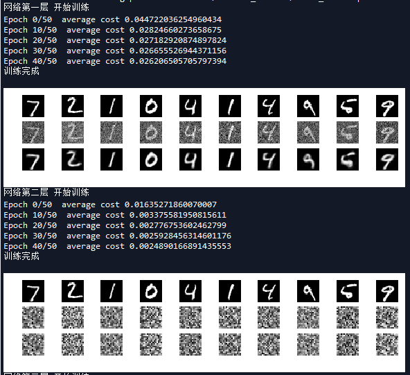
    训练 网络第一层
    '''
    with tf.Session() as sess:
        sess.run(tf.global_variables_initializer())
        #如果存在检查点文件 则恢复模型
        if kpt!=None:
            saver.restore(sess, kpt) 
        print('网络第一层 开始训练')
        for epoch in range(training_epochs):
            total_cost = 0.0
            for i in range(num_batch):
                batch_x,batch_y = mnist.train.next_batch(batch_size)
                #添加噪声 每次取出来一批次的数据，将输入数据的每一个像素都加上0.3倍的高斯噪声  
                batch_x_noise = batch_x + 0.3*np.random.randn(batch_size,784)  #标准正态分布
                _,loss = sess.run([l1_optm,l1_cost],feed_dict={x:batch_x_noise,y:batch_x,keep_prob:0.5})
                total_cost += loss
                
            #打印信息
            if epoch % display_epoch == 0:
                print('Epoch {0}/{1}  average cost {2}'.format(epoch,training_epochs,total_cost/num_batch))
                
            #每隔1轮后保存一次检查点            
            saver.save(sess,os.path.join(savedir,savefile),global_step = epoch)
        print('训练完成')
            
        #数据可视化                 
        test_noisy= mnist.test.images[:show_num]  + 0.3*np.random.randn(show_num,784)         
        reconstruction = sess.run(l1_reconstruction,feed_dict = {x:test_noisy,keep_prob:1.0})
        plt.figure(figsize=(1.0*show_num,1*2))        
        for i in range(show_num):
            #原始图像
            plt.subplot(3,show_num,i+1)            
            plt.imshow(np.reshape(mnist.test.images[i],(28,28)),cmap='gray')   
            plt.axis('off')
            #加入噪声后的图像
            plt.subplot(3,show_num,i+show_num*1+1)
            plt.imshow(np.reshape(test_noisy[i],(28,28)),cmap='gray')       
            plt.axis('off')
            #去燥自编码器输出图像
            plt.subplot(3,show_num,i+show_num*2+1)
            plt.imshow(np.reshape(reconstruction[i],(28,28)),cmap='gray')       
            plt.axis('off')
        plt.show()
    
    
    '''
    训练 网络第二层
    注意：这个网络模型的输入已经不再是MNIST图片了，而是上一层网络中的一层的输出
    '''
    with tf.Session() as sess:
        sess.run(tf.global_variables_initializer())
        print('网络第二层 开始训练')
        for epoch in range(training_epochs):
            total_cost = 0.0
            for i in range(num_batch):
                batch_x,batch_y = mnist.train.next_batch(batch_size)
                l1_out = sess.run(l1_h1,feed_dict={x:batch_x,keep_prob:1.0})
                                
                _,loss = sess.run([l2_optm,l2_cost],feed_dict={l2x:l1_out,l2y:l1_out})
                total_cost += loss
                
            #打印信息
            if epoch % display_epoch == 0:
                print('Epoch {0}/{1}  average cost {2}'.format(epoch,training_epochs,total_cost/num_batch))
                
            #每隔1轮后保存一次检查点            
            saver.save(sess,os.path.join(savedir,savefile),global_step = epoch)
        print('训练完成')
            
        #数据可视化                 
        testvec = mnist.test.images[:show_num]
        l1_out = sess.run(l1_h1,feed_dict={x:testvec,keep_prob:1.0})        
        reconstruction = sess.run(l2_reconstruction,feed_dict = {l2x:l1_out})
        plt.figure(figsize=(1.0*show_num,1*2))        
        for i in range(show_num):
            #原始图像
            plt.subplot(3,show_num,i+1)            
            plt.imshow(np.reshape(testvec[i],(28,28)),cmap='gray')   
            plt.axis('off')
            #加入噪声后的图像
            plt.subplot(3,show_num,i+show_num*1+1)
            plt.imshow(np.reshape(l1_out[i],(16,16)),cmap='gray')       
            plt.axis('off')
            #去燥自编码器输出图像
            plt.subplot(3,show_num,i+show_num*2+1)
            plt.imshow(np.reshape(reconstruction[i],(16,16)),cmap='gray')       
            plt.axis('off')
        plt.show()
    
    
    
    '''
    训练 网络第三层
    注意：同理这个网络模型的输入是要经过前面两次网络运算才可以生成
    '''
    with tf.Session() as sess:
        sess.run(tf.global_variables_initializer())
        print('网络第三层 开始训练')
        for epoch in range(training_epochs):
            total_cost = 0.0
            for i in range(num_batch):
                batch_x,batch_y = mnist.train.next_batch(batch_size)
                l1_out = sess.run(l1_h1,feed_dict={x:batch_x,keep_prob:1.0})
                l2_out = sess.run(l2_h1,feed_dict={l2x:l1_out})
                _,loss = sess.run([l3_optm,l3_cost],feed_dict={l3x:l2_out,l3y:batch_y})
                total_cost += loss
                
            #打印信息
            if epoch % display_epoch == 0:
                print('Epoch {0}/{1}  average cost {2}'.format(epoch,training_epochs,total_cost/num_batch))
                
            #每隔1轮后保存一次检查点            
            saver.save(sess,os.path.join(savedir,savefile),global_step = epoch)
        print('训练完成')
            

        '''
        栈式自编码网络验证 我们略过对第3层网络模型的单独验证，直接去验证整个分类模型，看看栈式自编码器的分类效果如何
        '''
        correct_prediction =tf.equal(tf.argmax(logits,1),tf.argmax(l3y,1))
        #计算准确率
        accuracy = tf.reduce_mean(tf.cast(correct_prediction,dtype=tf.float32))
        print('Accuracy:',accuracy.eval({x:mnist.test.images,l3y:mnist.test.labels}))
    
    
    '''
    级联微调
    将网络模型联起来进行分类训练
    '''
    with tf.Session() as sess:
        sess.run(tf.global_variables_initializer())
        print('级联微调 开始训练')
        for epoch in range(training_epochs):
            total_cost = 0.0
            for i in range(num_batch):
                batch_x,batch_y = mnist.train.next_batch(batch_size)            
                _,loss = sess.run([optm,cost],feed_dict={x:batch_x,l3y:batch_y})
                total_cost += loss
                
            #打印信息
            if epoch % display_epoch == 0:
                print('Epoch {0}/{1}  average cost {2}'.format(epoch,training_epochs,total_cost/num_batch))
            #每隔1轮后保存一次检查点            
            saver.save(sess,os.path.join(savedir,savefile),global_step = epoch)
        print('训练完成')
        print('Accuracy:',accuracy.eval({x:mnist.test.images,l3y:mnist.test.labels}))

运行结果如下：

可以看到，由于网络模型中各层的初始值已经训练好了，我们略过对第三层网络模型的单独验证，直接去验证整个分类模型，看看栈式自编码器的分类效果如何。可以看出直接将每层的训练参数堆起来，网络会有不错的表现，准确率达到86.97%。为了进一步优化，我们进行了级联微调，最终的准确率达到了97.74%。可以看到这个准确率和前馈神经网络准确度近似，但是我们可以增加网络的层数进一步提高准确率。

完整代码：

# -*- coding: utf-8 -*-
"""
Created on Wed May 30 20:21:43 2018

@author: zy
"""

'''
去燥自编码器和栈式自编码器的综合实现
1.我们首先建立一个去噪自编码器(包含输入层四层的网络)
2.然后再对第一层的输出做一次简单的自编码压缩(包含输入层三层的网络)
3.然后再将第二层的输出做一个softmax分类
4.最后把这3个网络里的中间层拿出来，组成一个新的网络进行微调1.构建一个包含输入层的简单去噪自编码其
'''

import tensorflow as tf
import numpy as np
import matplotlib.pyplot as plt
from tensorflow.examples.tutorials.mnist import input_data
import os

mnist = input_data.read_data_sets('../MNIST-data',one_hot=True)

print(type(mnist)) #<class 'tensorflow.contrib.learn.python.learn.datasets.base.Datasets'>

print('Training data shape:',mnist.train.images.shape)           #Training data shape: (55000, 784)
print('Test data shape:',mnist.test.images.shape)                #Test data shape: (10000, 784)
print('Validation data shape:',mnist.validation.images.shape)    #Validation data shape: (5000, 784)
print('Training label shape:',mnist.train.labels.shape)          #Training label shape: (55000, 10)

train_X = mnist.train.images
train_Y = mnist.train.labels
test_X = mnist.test.images
test_Y = mnist.test.labels


def stacked_auto_encoder():
    tf.reset_default_graph()
    '''
    栈式自编码器
    
    最终训练的一个网络为一个输入、一个输出和两个隐藏层
    MNIST输入(784) - > 编码层1(256)- > 编码层3(128) - > softmax分类
    
    除了输入层，每一层都用一个网络来训练，于是我们需要训练3个网络，最后再把训练好的各层组合在一起，形成第4个网络。
    '''
    
    
    '''
    网络参数定义
    '''
    n_input = 784
    n_hidden_1 = 256
    n_hidden_2 = 128
    n_classes = 10
    
    learning_rate = 0.01               #学习率
    training_epochs = 20               #迭代轮数
    batch_size = 256                   #小批量数量大小
    display_epoch = 10
    show_num = 10
    
    savedir = "./stacked_encoder/"     #检查点文件保存路径
    savefile = 'mnist_model.cpkt'      #检查点文件名
    
    #第一层输入
    x = tf.placeholder(dtype=tf.float32,shape=[None,n_input])
    y = tf.placeholder(dtype=tf.float32,shape=[None,n_input])
    keep_prob = tf.placeholder(dtype=tf.float32)
    
    #第二层输入
    l2x = tf.placeholder(dtype=tf.float32,shape=[None,n_hidden_1])
    l2y = tf.placeholder(dtype=tf.float32,shape=[None,n_hidden_1])
    
    #第三层输入
    l3x = tf.placeholder(dtype=tf.float32,shape=[None,n_hidden_2])
    l3y = tf.placeholder(dtype=tf.float32,shape=[None,n_classes])
    
    '''
    定义学习参数
    '''
    weights = {
            #网络1 784-256-256-784
            'l1_h1':tf.Variable(tf.truncated_normal(shape=[n_input,n_hidden_1],stddev=0.1)),    #级联使用
            'l1_h2':tf.Variable(tf.truncated_normal(shape=[n_hidden_1,n_hidden_1],stddev=0.1)),
            'l1_out':tf.Variable(tf.truncated_normal(shape=[n_hidden_1,n_input],stddev=0.1)),
            #网络2 256-128-128-256
            'l2_h1':tf.Variable(tf.truncated_normal(shape=[n_hidden_1,n_hidden_2],stddev=0.1)), #级联使用
            'l2_h2':tf.Variable(tf.truncated_normal(shape=[n_hidden_2,n_hidden_2],stddev=0.1)),
            'l2_out':tf.Variable(tf.truncated_normal(shape=[n_hidden_2,n_hidden_1],stddev=0.1)),
            #网络3 128-10
            'out':tf.Variable(tf.truncated_normal(shape=[n_hidden_2,n_classes],stddev=0.1))     #级联使用
            }
    
    biases = {
            #网络1 784-256-256-784
            'l1_b1':tf.Variable(tf.zeros(shape=[n_hidden_1])),       #级联使用
            'l1_b2':tf.Variable(tf.zeros(shape=[n_hidden_1])),
            'l1_out':tf.Variable(tf.zeros(shape=[n_input])),
            #网络2 256-128-128-256
            'l2_b1':tf.Variable(tf.zeros(shape=[n_hidden_2])),       #级联使用
            'l2_b2':tf.Variable(tf.zeros(shape=[n_hidden_2])),
            'l2_out':tf.Variable(tf.zeros(shape=[n_hidden_1])),
            #网络3 128-10
            'out':tf.Variable(tf.zeros(shape=[n_classes]))           #级联使用
            }
    
    '''
    定义第一层网络结构  
    注意：在第一层里加入噪声，并且使用弃权层 784-256-256-784
    '''
    l1_h1 = tf.nn.sigmoid(tf.add(tf.matmul(x,weights['l1_h1']),biases['l1_b1']))     
    l1_h1_dropout = tf.nn.dropout(l1_h1,keep_prob)
    l1_h2 = tf.nn.sigmoid(tf.add(tf.matmul(l1_h1_dropout,weights['l1_h2']),biases['l1_b2']))
    l1_h2_dropout = tf.nn.dropout(l1_h2,keep_prob)
    l1_reconstruction = tf.nn.sigmoid(tf.add(tf.matmul(l1_h2_dropout,weights['l1_out']),biases['l1_out']))
    
        
    #计算代价
    l1_cost = tf.reduce_mean((l1_reconstruction-y)**2)

    #定义优化器    
    l1_optm = tf.train.AdamOptimizer(learning_rate).minimize(l1_cost)
    
    
    '''
    定义第二层网络结构256-128-128-256
    '''
    l2_h1 = tf.nn.sigmoid(tf.add(tf.matmul(l2x,weights['l2_h1']),biases['l2_b1']))    
    l2_h2 = tf.nn.sigmoid(tf.add(tf.matmul(l2_h1,weights['l2_h2']),biases['l2_b2']))    
    l2_reconstruction = tf.nn.sigmoid(tf.add(tf.matmul(l2_h2,weights['l2_out']),biases['l2_out']))
    
        
    #计算代价
    l2_cost = tf.reduce_mean((l2_reconstruction-l2y)**2)

    #定义优化器    
    l2_optm = tf.train.AdamOptimizer(learning_rate).minimize(l2_cost)
    
    
    '''
    定义第三层网络结构 128-10
    '''    
    l3_logits = tf.add(tf.matmul(l3x,weights['out']),biases['out'])
    
        
    #计算代价
    l3_cost = tf.reduce_mean(tf.nn.softmax_cross_entropy_with_logits(logits=l3_logits,labels=l3y))

    #定义优化器    
    l3_optm = tf.train.AdamOptimizer(learning_rate).minimize(l3_cost)
    
    
    '''
    定义级联级网络结构
    
    将前三个网络级联在一起，建立第四个网络，并定义网络结构
    '''
    #1 联 2
    l1_l2_out = tf.nn.sigmoid(tf.add(tf.matmul(l1_h1,weights['l2_h1']),biases['l2_b1']))
    
    #2 联 3
    logits = tf.add(tf.matmul(l1_l2_out,weights['out']),biases['out'])
    
    #计算代价
    cost = tf.reduce_mean(tf.nn.softmax_cross_entropy_with_logits(logits=logits,labels=l3y))

    #定义优化器    
    optm = tf.train.AdamOptimizer(learning_rate).minimize(cost)
    
    num_batch = int(np.ceil(mnist.train.num_examples / batch_size))
    
    #生成Saver对象，max_to_keep = 1，表名最多保存一个检查点文件，这样在迭代过程中，新生成的模型就会覆盖以前的模型。
    saver = tf.train.Saver(max_to_keep=1) 
    
    #直接载入最近保存的检查点文件
    kpt = tf.train.latest_checkpoint(savedir)
    print("kpt:",kpt)    
    
    '''
    训练 网络第一层
    '''
    with tf.Session() as sess:
        sess.run(tf.global_variables_initializer())
        #如果存在检查点文件 则恢复模型
        if kpt!=None:
            saver.restore(sess, kpt) 
        print('网络第一层 开始训练')
        for epoch in range(training_epochs):
            total_cost = 0.0
            for i in range(num_batch):
                batch_x,batch_y = mnist.train.next_batch(batch_size)
                #添加噪声 每次取出来一批次的数据，将输入数据的每一个像素都加上0.3倍的高斯噪声  
                batch_x_noise = batch_x + 0.3*np.random.randn(batch_size,784)  #标准正态分布
                _,loss = sess.run([l1_optm,l1_cost],feed_dict={x:batch_x_noise,y:batch_x,keep_prob:0.5})
                total_cost += loss
                
            #打印信息
            if epoch % display_epoch == 0:
                print('Epoch {0}/{1}  average cost {2}'.format(epoch,training_epochs,total_cost/num_batch))
                
            #每隔1轮后保存一次检查点            
            saver.save(sess,os.path.join(savedir,savefile),global_step = epoch)
        print('训练完成')
            
        #数据可视化                 
        test_noisy= mnist.test.images[:show_num]  + 0.3*np.random.randn(show_num,784)         
        reconstruction = sess.run(l1_reconstruction,feed_dict = {x:test_noisy,keep_prob:1.0})
        plt.figure(figsize=(1.0*show_num,1*2))        
        for i in range(show_num):
            #原始图像
            plt.subplot(3,show_num,i+1)            
            plt.imshow(np.reshape(mnist.test.images[i],(28,28)),cmap='gray')   
            plt.axis('off')
            #加入噪声后的图像
            plt.subplot(3,show_num,i+show_num*1+1)
            plt.imshow(np.reshape(test_noisy[i],(28,28)),cmap='gray')       
            plt.axis('off')
            #去燥自编码器输出图像
            plt.subplot(3,show_num,i+show_num*2+1)
            plt.imshow(np.reshape(reconstruction[i],(28,28)),cmap='gray')       
            plt.axis('off')
        plt.show()
    
    
    '''
    训练 网络第二层
    注意：这个网络模型的输入已经不再是MNIST图片了，而是上一层网络中的一层的输出
    '''
    with tf.Session() as sess:
        sess.run(tf.global_variables_initializer())
        print('网络第二层 开始训练')
        for epoch in range(training_epochs):
            total_cost = 0.0
            for i in range(num_batch):
                batch_x,batch_y = mnist.train.next_batch(batch_size)
                l1_out = sess.run(l1_h1,feed_dict={x:batch_x,keep_prob:1.0})
                                
                _,loss = sess.run([l2_optm,l2_cost],feed_dict={l2x:l1_out,l2y:l1_out})
                total_cost += loss
                
            #打印信息
            if epoch % display_epoch == 0:
                print('Epoch {0}/{1}  average cost {2}'.format(epoch,training_epochs,total_cost/num_batch))
                
            #每隔1轮后保存一次检查点            
            saver.save(sess,os.path.join(savedir,savefile),global_step = epoch)
        print('训练完成')
            
        #数据可视化                 
        testvec = mnist.test.images[:show_num]
        l1_out = sess.run(l1_h1,feed_dict={x:testvec,keep_prob:1.0})        
        reconstruction = sess.run(l2_reconstruction,feed_dict = {l2x:l1_out})
        plt.figure(figsize=(1.0*show_num,1*2))        
        for i in range(show_num):
            #原始图像
            plt.subplot(3,show_num,i+1)            
            plt.imshow(np.reshape(testvec[i],(28,28)),cmap='gray')   
            plt.axis('off')
            #加入噪声后的图像
            plt.subplot(3,show_num,i+show_num*1+1)
            plt.imshow(np.reshape(l1_out[i],(16,16)),cmap='gray')       
            plt.axis('off')
            #去燥自编码器输出图像
            plt.subplot(3,show_num,i+show_num*2+1)
            plt.imshow(np.reshape(reconstruction[i],(16,16)),cmap='gray')       
            plt.axis('off')
        plt.show()
    
    
    
    '''
    训练 网络第三层
    注意：同理这个网络模型的输入是要经过前面两次网络运算才可以生成
    '''
    with tf.Session() as sess:
        sess.run(tf.global_variables_initializer())
        print('网络第三层 开始训练')
        for epoch in range(training_epochs):
            total_cost = 0.0
            for i in range(num_batch):
                batch_x,batch_y = mnist.train.next_batch(batch_size)
                l1_out = sess.run(l1_h1,feed_dict={x:batch_x,keep_prob:1.0})
                l2_out = sess.run(l2_h1,feed_dict={l2x:l1_out})
                _,loss = sess.run([l3_optm,l3_cost],feed_dict={l3x:l2_out,l3y:batch_y})
                total_cost += loss
                
            #打印信息
            if epoch % display_epoch == 0:
                print('Epoch {0}/{1}  average cost {2}'.format(epoch,training_epochs,total_cost/num_batch))
                
            #每隔1轮后保存一次检查点            
            saver.save(sess,os.path.join(savedir,savefile),global_step = epoch)
        print('训练完成')
            

        '''
        栈式自编码网络验证
        '''
        correct_prediction =tf.equal(tf.argmax(logits,1),tf.argmax(l3y,1))
        #计算准确率
        accuracy = tf.reduce_mean(tf.cast(correct_prediction,dtype=tf.float32))
        print('Accuracy:',accuracy.eval({x:mnist.test.images,l3y:mnist.test.labels}))
    
    
    '''
    级联微调
    将网络模型联起来进行分类训练
    '''
    with tf.Session() as sess:
        sess.run(tf.global_variables_initializer())
        print('级联微调 开始训练')
        for epoch in range(training_epochs):
            total_cost = 0.0
            for i in range(num_batch):
                batch_x,batch_y = mnist.train.next_batch(batch_size)            
                _,loss = sess.run([optm,cost],feed_dict={x:batch_x,l3y:batch_y})
                total_cost += loss
                
            #打印信息
            if epoch % display_epoch == 0:
                print('Epoch {0}/{1}  average cost {2}'.format(epoch,training_epochs,total_cost/num_batch))
            #每隔1轮后保存一次检查点            
            saver.save(sess,os.path.join(savedir,savefile),global_step = epoch)
        print('训练完成')
        print('Accuracy:',accuracy.eval({x:mnist.test.images,l3y:mnist.test.labels}))

        
if  __name__ == '__main__':
    stacked_auto_encoder()