

Python数据分析第三周作业随笔
第一部分——飞机客户数据分析预测
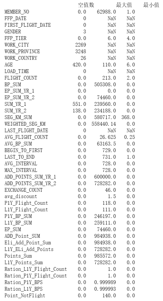
代码一:数据探索
#代码7-1 数据探索
#对数据进行基本的探索
#返回缺失值个数以及最大、最小值
import pandas as pd
datafile = "D:\\360MoveData\\Users\\86130\\Documents\\Tencent Files\\2268756693\\FileRecv\\air_data(1).csv"# 航空原始数据,第一行为属性标签
resultfile = "D:\\360MoveData\\Users\\86130\\Documents\\Tencent Files\\2268756693\\FileRecv\\explore.csv"# 数据探索结果表

# 读取原始数据,指定UTF-8编码(需要用文本编辑器将数据转换为UTF-8编码)
data = pd.read_csv(datafile,encoding = 'utf-8')

# 包括对数据的基本描述,percentiles参数是指定计算多少的分位数表(如¼分位数、中位数等)
explore = data.describe(percentiles = [] ,include = 'all').T
# describe()函数自动计算非空值数,需要手动计算空值数
explore['null'] = len(data)-explore['count']

explore = explore[['null','max','min']]
#explore.columns = [u'空值数',u'最大值',u'最小值'] #表头重命名
'''
这里只选取部分探索结果。
describe()函数自动计算的字段有count(非空值数)、unique(唯一值数)、top(频数最高者)、
freq(最高频数)、mean(平均值)、std(方差)、min(最小值)、50%(中位数)、max(最大值)
'''

explore.to_csv(resultfile) #导出结果
代码二:分析数据并绘制基本图像
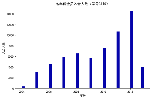
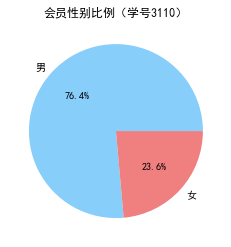
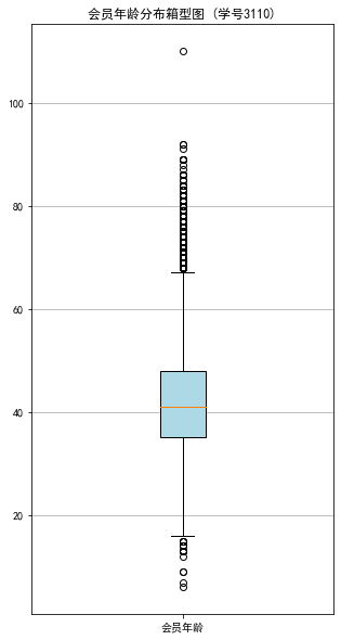
#代码7-2 探索客户的基本信息分布情况
#客户信息类别
#提取会员入会年份
import pandas as pd
import matplotlib.pyplot as plt
from datetime import datetime
ffp = data['FFP_DATE'].apply(lambda x:datetime.strptime(x,'%Y/%m/%d'))
ffp_year = ffp.map(lambda x : x.year)
#绘制各年份会员入会人数直方图
fig = plt.figure(figsize=(8,5)) # 设置画布大小
plt.rcParams['font.sans-serif'] = 'SimHei' #设置中文显示
plt.rcParams['axes.unicode_minus'] = False
plt.hist(ffp_year,bins='auto',color='#0504aa')
plt.xlabel('年份')
plt.ylabel('入会人数')
plt.title('各年份会员入会人数(学号3110)')
plt.show()
plt.close

#提取会员不同性别人数
male = pd.value_counts(data['GENDER'])['男']
female = pd.value_counts(data['GENDER'])['女']
#绘制会员性别比例饼图
fig = plt.figure(figsize=(7,4)) #设置画布大小
plt.pie([male,female],labels=['男','女'],colors=['lightskyblue','lightcoral'],autopct='%1.1f%%')
plt.title('会员性别比例(学号3110)')
plt.show()
plt.close

#提取不同级别会员的人数
lv_four = pd.value_counts(data['FFP_TIER'])[4]
lv_five = pd.value_counts(data['FFP_TIER'])[5]
lv_six = pd.value_counts(data['FFP_TIER'])[6]

#绘制会员各级别人数条形图
fig = plt.figure(figsize=(8,5)) #设置画布大小
plt.bar(x=range(3),height=[lv_four,lv_five,lv_six],width=0.4,alpha=0.8,color='skyblue')
plt.xticks([index for index in range(3)],['4','5','6'])

plt.xlabel('会员等级')
plt.ylabel('会员人数')
plt.title('会员各级别人数 (学号3110)')
plt.show()
plt.close

# 提取会员年龄
age = data['AGE'].dropna()
age = age.astype('int64')
# 绘图会员年龄分布箱型图
fig = plt.figure(figsize=(5, 10))
plt.boxplot(age,
           patch_artist=True,
           labels = ['会员年龄'],   # 设置x轴标题
           boxprops = {'facecolor':'lightblue'}) # 设置填充颜色
plt.title('会员年龄分布箱型图 (学号3110)')
# 显示y坐标的底线
plt.grid(axis='y')
plt.show()
plt.close

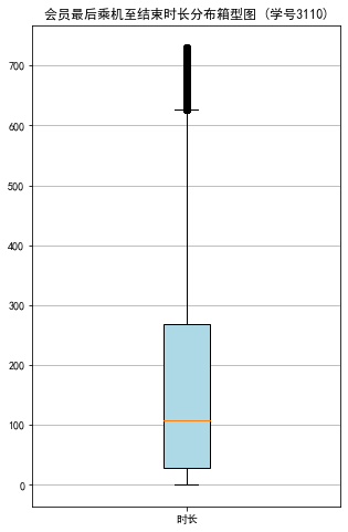
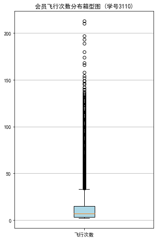
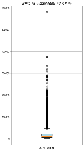
代码三:客户乘机数据分析箱型图
#代码7-3 探索客户乘机信息分布情况
import matplotlib.pyplot as plt
lte =data['LAST_TO_END']
fc = data['FLIGHT_COUNT']
sks = data['SEG_KM_SUM']

#绘制最后乘机至结束时长箱型图
fig = plt.figure(figsize=(5,8))

plt.boxplot(lte,
            patch_artist=True,
           labels = ['时长'], #设置x轴标题
           boxprops = {'facecolor':'lightblue'}) #设置填充颜色
plt.title('会员最后乘机至结束时长分布箱型图 (学号3110)')
#显示y坐标轴的底线
plt.grid(axis='y')
plt.show()
plt.close

#绘制客户飞行次数箱型图
fig = plt.figure(figsize=(5,8))
plt.boxplot(fc,
            patch_artist=True,
           labels = ['飞行次数'], #设置x轴标题
           boxprops = {'facecolor':'lightblue'}) #设置填充颜色
plt.title('会员飞行次数分布箱型图 (学号3110)')
# 显示y坐标的底线
plt.grid(axis='y')
plt.show()
plt.close

# 绘制客户总飞行公里数箱型图
fig = plt.figure(figsize=(5,10))
plt.boxplot(sks,
           patch_artist=True,
           labels = ['总飞行公里数'],   # 设置x轴标题
           boxprops = {'facecolor':'lightblue'}) # 设置填充颜色
plt.title('客户总飞行公里数箱型图 (学号3110)')
# 显示y坐标的底线
plt.grid(axis='y')
plt.show()
plt.close
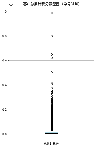
代码四:会员积分数据分析直方图
#代码7-4 探索客户积分信息分布情况
import matplotlib.pyplot as plt
ec = data['EXCHANGE_COUNT']
#绘制会员兑换积分次数直方图
fig = plt.figure(figsize=(8,5)) #设置画布大小
plt.hist(ec,bins=5,color='#0504aa')
plt.xlabel('兑换次数')
plt.ylabel('会员人数')
plt.title('会员兑换积分次数分布直方图 (学号3110)')
plt.show()
plt.close

#提取会员总累计积分
ps = data['Points_Sum']
#绘制会员总累计积分箱型图
fig = plt.figure(figsize=(5,8))
plt.boxplot(ps,
            patch_artist=True,
           labels = ['总累计积分'], #设置x轴标题
           boxprops = {'facecolor':'lightblue'}) #设置填充颜色
plt.title('客户总累计积分箱型图 (学号3110)')
# 显示y坐标的底线
plt.grid(axis='y')
plt.show()
plt.close

代码五:相关矩阵及热力图
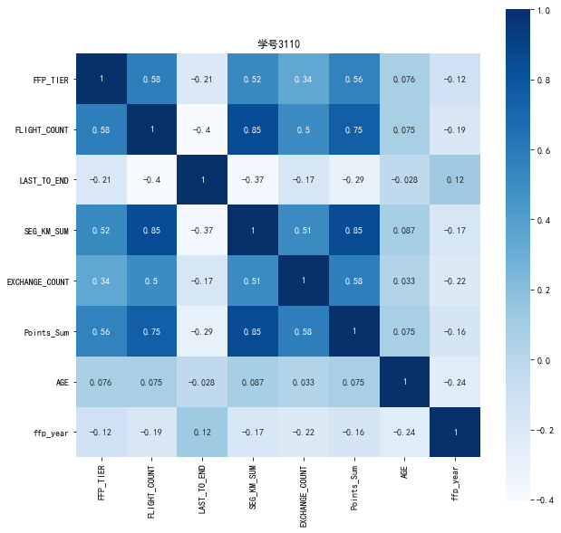
#代码7-5 相关系数矩阵与热力图
data_corr = data[['FFP_TIER','FLIGHT_COUNT','LAST_TO_END','SEG_KM_SUM','EXCHANGE_COUNT','Points_Sum']]
age1 = data['AGE'].fillna(0)
data_corr['AGE'] = age1.astype('int64')
data_corr['ffp_year'] = ffp_year

#计算相关性矩阵
dt_corr = data_corr.corr(method='pearson')
print('相关性矩阵为:\n',dt_corr)

#绘制热力图
import seaborn as sns
plt.subplots(figsize=(10,10)) #设置画面大小
sns.heatmap(dt_corr,annot=True,vmax=1,square=True,cmap='Blues')
plt.title('学号3110')
plt.show()
plt.close
相关性矩阵为:
                 FFP_TIER  FLIGHT_COUNT  LAST_TO_END  SEG_KM_SUM  \
FFP_TIER        1.000000      0.582447    -0.206313    0.522350
FLIGHT_COUNT    0.582447      1.000000    -0.404999    0.850411
LAST_TO_END    -0.206313     -0.404999     1.000000   -0.369509
SEG_KM_SUM      0.522350      0.850411    -0.369509    1.000000
EXCHANGE_COUNT  0.342355      0.502501    -0.169717    0.507819
Points_Sum      0.559249      0.747092    -0.292027    0.853014
AGE             0.076245      0.075309    -0.027654    0.087285
ffp_year       -0.116510     -0.188181     0.117913   -0.171508

                EXCHANGE_COUNT  Points_Sum       AGE  ffp_year
FFP_TIER              0.342355    0.559249  0.076245 -0.116510
FLIGHT_COUNT          0.502501    0.747092  0.075309 -0.188181
LAST_TO_END          -0.169717   -0.292027 -0.027654  0.117913
SEG_KM_SUM            0.507819    0.853014  0.087285 -0.171508
EXCHANGE_COUNT        1.000000    0.578581  0.032760 -0.216610
Points_Sum            0.578581    1.000000  0.074887 -0.163431
AGE                   0.032760    0.074887  1.000000 -0.242579
ffp_year             -0.216610   -0.163431 -0.242579  1.000000
代码六:进行数据清洗
#代码7-6 清洗空值与异常值
import numpy as np
import pandas as pd

datafile = "D:\\360MoveData\\Users\\86130\\Documents\\Tencent Files\\2268756693\\FileRecv\\air_data(1).csv"
cleanedfile = "D:\\360MoveData\\Users\\86130\\Documents\\Tencent Files\\2268756693\\FileRecv\\data_cleaned.csv"

#读取数据
airline_data = pd.read_csv(datafile,encoding = 'utf-8')
print('原始数据的形状为:',airline_data.shape)

#去除票价为空的记录
airline_notnull = airline_data.loc[airline_data['SUM_YR_1'].notnull() &
                                  airline_data['SUM_YR_2'].notnull(),:]
print('删除缺失记录后数据的形状为:',airline_notnull.shape)

# 只保留票价非零的,或者平均折扣率不为0且总飞行公里数大于0的记录
index1 = airline_notnull['SUM_YR_1'] != 0
index2 = airline_notnull['SUM_YR_2'] != 0
index3 = (airline_notnull['SEG_KM_SUM']>0) & (airline_notnull['avg_discount'] != 0)
index4 = airline_notnull['AGE'] >100 # 去除年龄大于100的记录
airline = airline_notnull[(index1 | index2) & index3 & ~index4]
print('数据清洗后数据的形状为:', airline.shape)

airline.to_csv(cleanedfile) # 保存清洗后的数据
原始数据的形状为: (62988, 44)
删除缺失记录后数据的形状为: (62299, 44)
数据清洗后数据的形状为: (62043, 44)

代码七:属性选择
# 代码7-7 属性选择
import pandas as pd
import numpy as np

# 读取数据清洗后的数据
cleanedfile = "D:\\360MoveData\\Users\\86130\\Documents\\Tencent Files\\2268756693\\FileRecv\\data_cleaned.csv" # 数据清洗后保存的文件路径
airline = pd.read_csv(cleanedfile, encoding='utf-8')
# 选取需求属性
airline_selection = airline[['FFP_DATE', 'LOAD_TIME', 'LAST_TO_END', 'FLIGHT_COUNT', 'SEG_KM_SUM', 'avg_discount']]
print('筛选的属性前5行为:\n', airline_selection.head())
筛选的属性前5行为:
     FFP_DATE  LOAD_TIME  LAST_TO_END  FLIGHT_COUNT  SEG_KM_SUM  avg_discount
0  2006/11/2  2014/3/31            1           210      580717      0.961639
1  2007/2/19  2014/3/31            7           140      293678      1.252314
2   2007/2/1  2014/3/31           11           135      283712      1.254676
3  2008/8/22  2014/3/31           97            23      281336      1.090870
4  2009/4/10  2014/3/31            5           152      309928      0.970658

代码八:属性构造与数据标准化
# 代码7-8 属性构造与数据标准化
# 构造属性L
L = pd.to_datetime(airline_selection['LOAD_TIME']) -  pd.to_datetime(airline_selection['FFP_DATE'])
L = L.astype('str').str.split().str[0]
L = L.astype('int')/30

# 合并属性
airline_features = pd.concat([L,airline_selection.iloc[:,2:]],axis=1)
print('构建的LRFMC属性前5行为:\n', airline_features.head())

# 数据标准化
from sklearn.preprocessing import StandardScaler
data = StandardScaler().fit_transform(airline_features)
np.savez("D:\\360MoveData\\Users\\86130\\Documents\\Tencent Files\\2268756693\\FileRecv\\airline_scale.npz", data)
print('标准化后LRFMC 5个属性为:\n', data[:5,:])
构建的LRFMC属性前5行为:
            0  LAST_TO_END  FLIGHT_COUNT  SEG_KM_SUM  avg_discount
0  90.200000            1           210      580717      0.961639
1  86.566667            7           140      293678      1.252314
2  87.166667           11           135      283712      1.254676
3  68.233333           97            23      281336      1.090870
4  60.533333            5           152      309928      0.970658
标准化后LRFMC 5个属性为:
 [[ 1.43579256 -0.94493902 14.03402401 26.76115699  1.29554188]
 [ 1.30723219 -0.91188564  9.07321595 13.12686436  2.86817777]
 [ 1.32846234 -0.88985006  8.71887252 12.65348144  2.88095186]
 [ 0.65853304 -0.41608504  0.78157962 12.54062193  1.99471546]
 [ 0.3860794  -0.92290343  9.92364019 13.89873597  1.34433641]]
代码九:K-Meas聚类标准化后的数据
#代码7-9 K-Meas聚类标准化后的数据
import pandas as pd
import numpy as np
from sklearn.cluster import KMeans #导入K-Mmeans算法

#读取标准化后的数据
airline_scale = np.load("D:\\360MoveData\\Users\\86130\\Documents\\Tencent Files\\2268756693\\FileRecv\\airline_scale.npz")['arr_0']
k = 5 #确定聚类中心数

#构建模型,随机种子设为123
kmeans_model = KMeans(n_clusters=k,random_state=123)
fit_kmeans = kmeans_model.fit(airline_scale) #模型训练

#查看聚类结果
kmeans_cc = kmeans_model.cluster_centers_ #聚类中心
print('各聚类中心为:\n',kmeans_cc)
kmeans_labels = kmeans_model.labels_ #样本的类别标签
print('各样本的类别标签为:\n',kmeans_labels)
r1 = pd.Series(kmeans_model.labels_).value_counts() #统计不同类别样本的数目
print('最终每个类别的数目为:\n',r1)
#输出聚类分群的结果
cluster_center = pd.DataFrame(kmeans_model.cluster_centers_,\
                             columns = ['ZL','ZR','ZF','ZM','ZC']) #将聚类中心放在数据中
cluster_center.index = pd.DataFrame(kmeans_model.labels_).\
                             drop_duplicates().iloc[:,0] #将样本类别作为数据框索引
print(cluster_center)
各聚类中心为:
 [[-0.70030628 -0.41502288 -0.16081841 -0.16053724 -0.25728596]
 [ 0.0444681  -0.00249102 -0.23046649 -0.23492871  2.17528742]
 [ 0.48370858 -0.79939042  2.48317171  2.42445742  0.30923962]
 [ 1.1608298  -0.37751261 -0.08668008 -0.09460809 -0.15678402]
 [-0.31319365  1.68685465 -0.57392007 -0.5367502  -0.17484815]]
各样本的类别标签为:
 [2 2 2 ... 0 4 4]
最终每个类别的数目为:
 0    24630
3    15733
4    12117
2     5337
1     4226
dtype: int64
         ZL        ZR        ZF        ZM        ZC
0
2 -0.700306 -0.415023 -0.160818 -0.160537 -0.257286
1  0.044468 -0.002491 -0.230466 -0.234929  2.175287
3  0.483709 -0.799390  2.483172  2.424457  0.309240
0  1.160830 -0.377513 -0.086680 -0.094608 -0.156784
4 -0.313194  1.686855 -0.573920 -0.536750 -0.174848
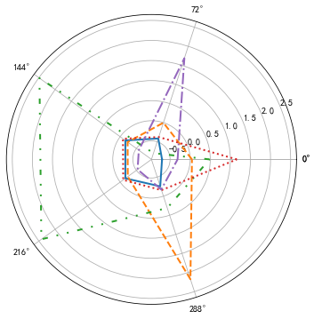
代码十:绘制客户分群雷达图
# 代码7-10 绘制客户分群雷达图
%matplotlib inline
import matplotlib.pyplot as plt
import pandas as pd
import numpy as np
from sklearn.cluster import KMeans #导入K-Mmeans算法
# 客户分群雷达图
labels = ['ZL','ZR','ZF','ZM','ZC']
legen = ['客户群' + str(i + 1) for i in cluster_center.index] # 客户群命名
lstype = ['-', '--', (0, (3,5,1,5,1,5)), ':', '-.']
kinds = list(cluster_center.iloc[:, 0])
# 由于雷达图要保证数据闭合,因此再添加L列,并转换为np.ndarray
cluster_center = pd.concat([cluster_center, cluster_center[['ZL']]], axis=1)
centers = np.array(cluster_center.iloc[:, 0:])

# 分割圆周长,并让其闭合
n = len(labels)
angle = np.linspace(0, 2*np.pi, n, endpoint=False)
angle = np.concatenate((angle, [angle[0]]))

#绘图
fig = plt.figure(figsize=(8,6))
ax = fig.add_subplot(111,polar=True) #以极坐标的形式绘制图形
plt.rcParams['font.sans-serif'] = 'SimHei' #设置中文显示
plt.rcParams['axes.unicode_minus'] = False #用来正常显示负号
#画线
for i in range(len(kinds)):
    ax.plot(angle,centers[i],linestyle=lstype[i],linewidth=2,label=kinds[i])
#添加属性标签
ax.set_thetagrids(angle * 180 / np.pi,labels)
plt.title('客户特征分析雷达图(学号3110)')
plt.legend(legen)
plt.show()
plt.close
![]()
第二部分:电信客户流失分析预测
代码1:读取并简单分析数据
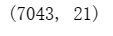
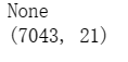
import pandas as pd
data=pd.read_csv('D:\大三下大数据分析\课堂练习第三周\客户流失数据\\WA_Fn-UseC_-Telco-Customer-Churn.csv')# 加载数据
data.shape  # 查看数据大小
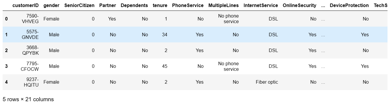
data.head()
data.dtypes# 查看数据类型
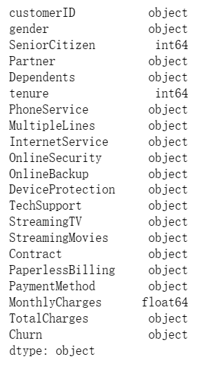
data.info() # 打印摘要

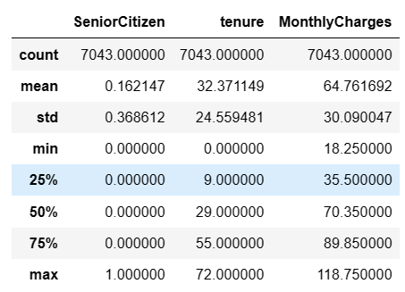
data.describe() # 描述性统计信息
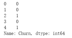
代码2:客户流失数据分析
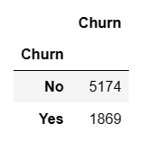
User_info=data.groupby(by="Churn")["Churn"].count()
User_info=pd.DataFrame(User_info)
User_info
代码3:查看数据类型
print(telcon.info()) #查看数据类型
<class 'pandas.core.frame.DataFrame'>
RangeIndex: 7043 entries, 0 to 7042
Data columns (total 21 columns):
 #   Column            Non-Null Count  Dtype
---  ------            --------------  -----
 0   customerID        7043 non-null   object
 1   gender            7043 non-null   object
 2   SeniorCitizen     7043 non-null   int64
 3   Partner           7043 non-null   object
 4   Dependents        7043 non-null   object
 5   tenure            7043 non-null   int64
 6   PhoneService      7043 non-null   object
 7   MultipleLines     7043 non-null   object
 8   InternetService   7043 non-null   object
 9   OnlineSecurity    7043 non-null   object
 10  OnlineBackup      7043 non-null   object
 11  DeviceProtection  7043 non-null   object
 12  TechSupport       7043 non-null   object
 13  StreamingTV       7043 non-null   object
 14  StreamingMovies   7043 non-null   object
 15  Contract          7043 non-null   object
 16  PaperlessBilling  7043 non-null   object
 17  PaymentMethod     7043 non-null   object
 18  MonthlyCharges    7043 non-null   float64
 19  TotalCharges      7043 non-null   object
 20  Churn             7043 non-null   object
dtypes: float64(1), int64(2), object(18)
memory usage: 1.1+ MB
None
代码4:处理缺失值和归一化处理
#TotalCharges表示总费用,这里为对象类型,需要转换为float类型
'''
convert_numeric=True表示强制转换数字(包括字符串),不可转换为NaN---已被弃用
您可以根据需要替换所有非数字值,以NaN使用with函数中的apply列,然后替换为by 并将所有值最后替换为s by :
df to_numeric 0 fillna int astype
'''
data['TotalCharges']=data['TotalCharges'].apply(pd.to_numeric, errors='coerce').fillna(0).astype(int)
print(data['TotalCharges'].dtypes)
#
print(pd.isnull(data['TotalCharges']).sum()) #再次查找是否存在缺失值

#处理缺失值

print(data.dropna(inplace=True)) #删除掉缺失值所在的行
print(data.shape)
#数据归一化处理
#对Churn列中的YES和No分别用1和0替换,方便后续处理
data['Churn'].replace(to_replace='Yes',value=1,inplace=True)
data['Churn'].replace(to_replace='No',value=0,inplace=True)
print(data['Churn'].head())
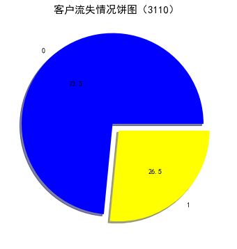
代码5:绘制客户流失情况饼图
#查看流失客户占比

churnvalue=telcon[ "Churn" ].value_counts()
labels=telcon["Churn"].value_counts().index

rcParams["figure.figsize"]=6,6
plt.pie(churnvalue,labels=labels,colors=["blue","yellow"],explode=(0.1,0),autopct='%1.1f', shadow=True)
plt.title( '客户流失情况饼图(3110) ',fontsize=15)
plt.rcParams['font.sans-serif'] = 'SimHei' #设置中文显示
plt.show()
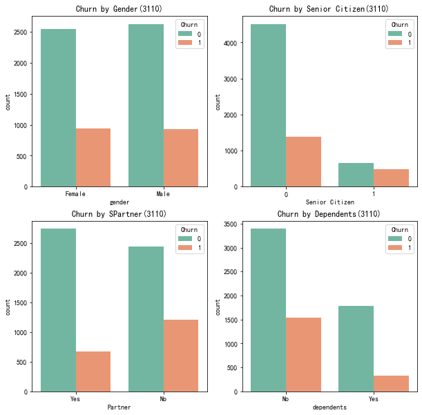
代码6:客户流失影响直方图
#性别、老年人、配偶、亲属对流客户流失率的影响

plt.figure(figsize=(10,10))
plt.subplot(2,2,1)
gender=sns.countplot(x='gender',hue='Churn',data=telcon,palette='Set2')   #palette参数表示设置颜色,设置为主颜色paste12
plt.xlabel('gender')
plt.title('Churn by Gender(3110)')

plt.subplot(2,2,2)
seniorcitizen=sns.countplot(x='SeniorCitizen',hue='Churn',data=telcon,palette='Set2')
plt.xlabel('Senior Citizen')
plt.title('Churn by Senior Citizen(3110)')

plt.subplot(2,2,3)
partner=sns.countplot(x='Partner',hue='Churn',data=telcon,palette='Set2')
plt.xlabel('Partner')
plt.title('Churn by SPartner(3110)')

plt.subplot(2,2,4)
dependents=sns.countplot(x='Dependents',hue='Churn',data=telcon,palette='Set2')
plt.xlabel('dependents')
plt.title('Churn by Dependents(3110)')
plt.show()
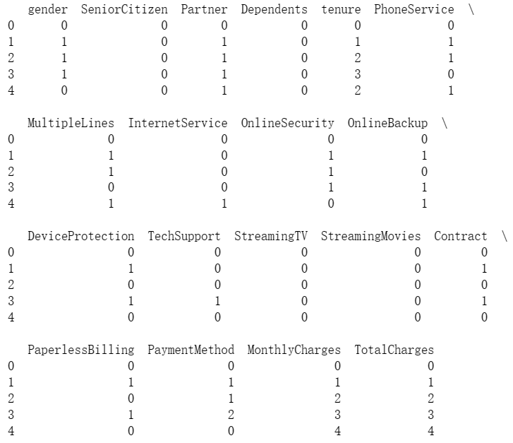
代码7:特征值
charges=telcon.iloc[:,1:20]
# #对特征进行编码
# #离散特征的编码分为两种情况:
# #1.离散特征的取值之间没有太大意义,比如color:[red,blue],那么就使用one-hot编码
# #2.离散特征的取值有大小意义,比如size:[X,XL,XXL],那么就使用数值的映射【X:1,XL:2,XXL:3】
corrdf=charges.apply(lambda x:pd.factorize(x)[0])
print(corrdf.head())
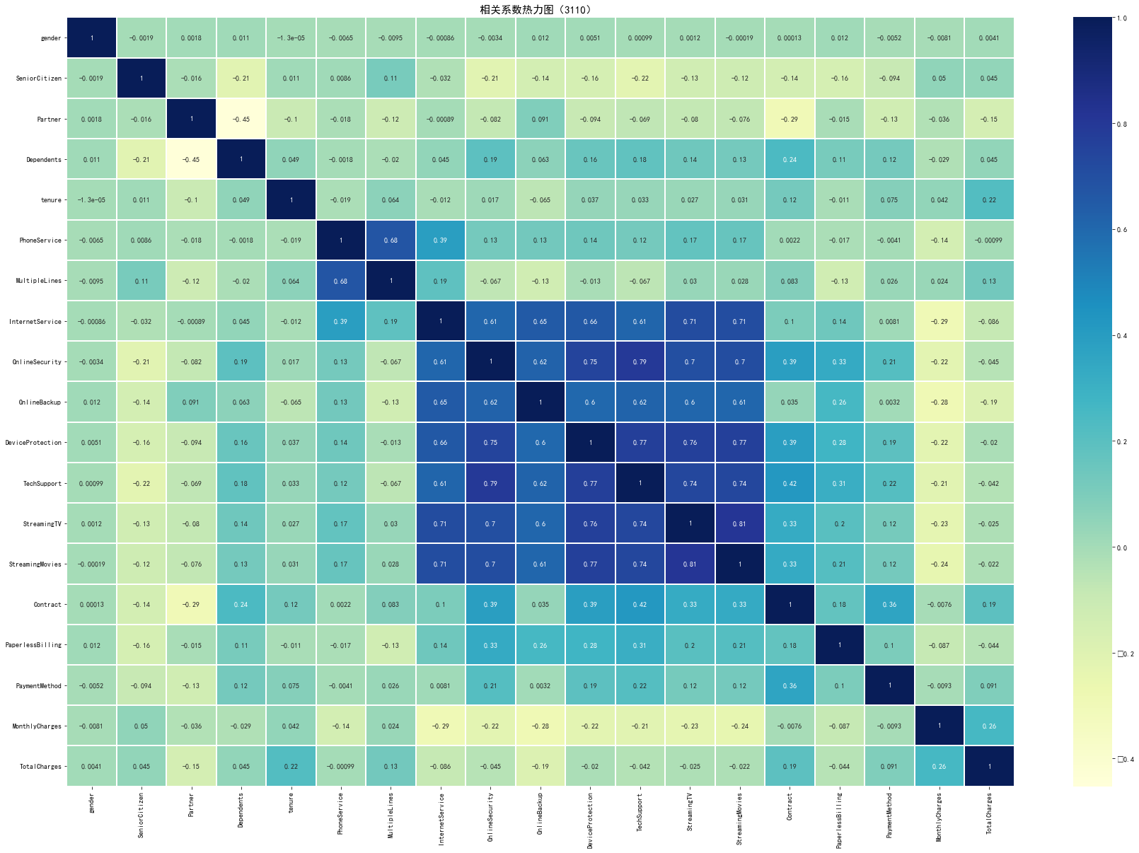
代码8:热力图
#使用热地图显示相关系数

charges=telcon.iloc[:,1:20]
corrdf=charges.apply(lambda x:pd.factorize(x)[0])
corr=corrdf.corr()
# '''
# heatmap 使用热力图展示系数矩阵情况
# linewidths 热力图矩阵之间的间隔大小
# annot  设定是否显示每个色块系数值
# '''
plt.figure(figsize=(30,20))
ax=sns.heatmap(corr,xticklabels=corr.columns,yticklabels=corr.columns,linewidths=0.2,cmap='YlGnBu',annot=True)
plt.title('相关系数热力图(3110) ',fontsize=15)
plt.rcParams['font.sans-serif'] = 'SimHei' #设置中文显示
plt.show()
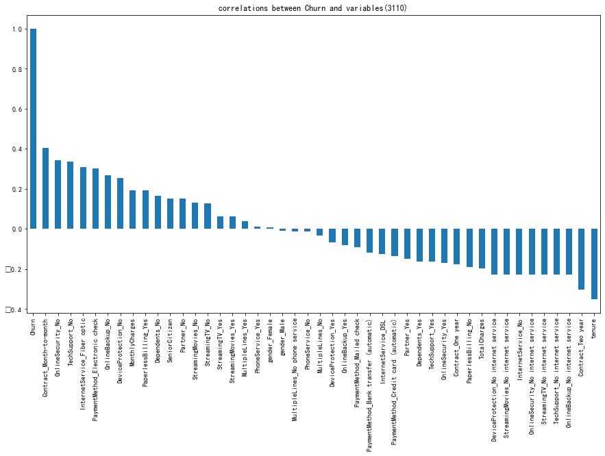
代码9:电信用户是否流失与各变量之间的相关性
#电信用户是否流失与各变量之间的相关性

plt.figure(figsize=(15,8))
tel_dummies.corr()['Churn'].sort_values(ascending=False).plot(kind='bar')
plt.title('correlations between Churn and variables(3110)')
plt.show()
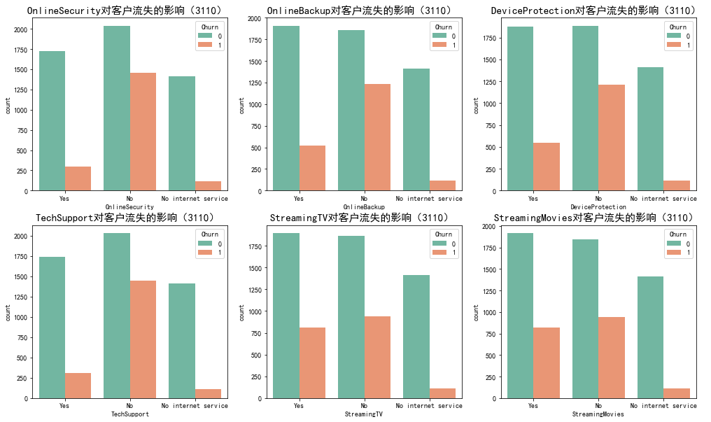
代码10:网络安全服务、在线备份业务、设备保护业务、技术支持服务、网络电视、网络电影和无互联网服务对客户流失率的影响
#网络安全服务、在线备份业务、设备保护业务、技术支持服务、网络电视、网络电影和无互联网服务对客户流失率的影响

covariable=['OnlineSecurity','OnlineBackup','DeviceProtection','TechSupport','StreamingTV','StreamingMovies']
plt.figure(figsize=(17,10))
for i,item in enumerate(covariable):
    plt.subplot(2,3,(i+1))
    ax=sns.countplot(x=item,hue='Churn',data=telcon,palette='Set2',order=['Yes','No','No internet service'])
    plt.xlabel(str(item))
    plt.title(str(item)+'对客户流失的影响(3110) ',fontsize=15)
    i=i+1
plt.show()
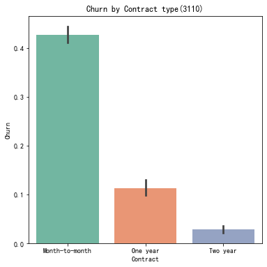
代码11:绘制签订合同方式对客户流失率的影响直方图
#签订合同方式对客户流失率的影响

ax=sns.barplot(x='Contract',y='Churn',data=telcon,palette='Set2',order=['Month-to-month','One year','Two year'])
# seaborn 的 barplot() 利用矩阵条的高度反映数值变量的集中趋势,bar plot 展示的是某种变量分布的平均值,
# 当需要精确观察每类变量的分布趋势,boxplot 与 violinplot 往往是更好的选择。
plt.title('Churn by Contract type(3110)')
plt.show()
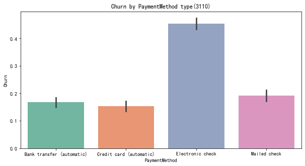
代码12:绘制付款方式对客户流失率的影响直方图
#付款方式对客户流失率的影响

plt.figure(figsize=(10,5))
ax=sns.barplot(x='PaymentMethod',y='Churn',data=telcon,palette='Set2',order=['Bank transfer (automatic)','Credit card (automatic)','Electronic check','Mailed check'])
plt.title('Churn by PaymentMethod type(3110)')
plt.show()

 浙公网安备 33010602011771号