线性回归算法
简介
- 解决回归问题
- 思想简单,实现容易
- 许多强大的非线性模型的基础
- 结果具有很好的可解释性
- 蕴含机器学习中的很多重要思想
线性回归算法以一个坐标系里一个维度为结果,其他维度为特征(如二维平面坐标系中横轴为特征,纵轴为结果),无数的训练集放在坐标系中,发现他们是围绕着一条执行分布。线性回归算法的期望,就是寻找一条直线,最大程度的“拟合”样本特征和样本输出标记的关系
简单线性回归
模型
被用来描述因变量X与自变量Y以及偏差之间的关系的方程称为回归模型简单线性回归的模型如下:
$y=ax+b+\varepsilon $
$a$:回归线斜率,表示X每增加1单位所引起Y的增量
$b$:回归系数,回归线有纵轴上的截距
$\varepsilon$:Y与回归线的平均数间的误差,随机变量,服从正态分布
由于母体回归线无法得知,无法得到真实的斜率截距,可以采用样本回归线估计值,对于每一个样本点 $x^{i}$
预测值为:$\widehat{y}^{i}=ax^{i}+b$
真实值为:$y^{i}$
我们希望 $y^{i}$和$\widehat{y}^{i}$ 的差距尽量小,故使 $\sum_{i=1}^{m}(y^{i}-\widehat{y}^{i})^{2}$ 尽可能小,则有
$\widehat{y}^{i}=ax^{i}+b$
$a=\frac{\sum_{i=1}^{m}(x^{i}-\overline{x})(y^{i}-\overline{y})}{\sum_{i=1}^{m}(x^{i}-\overline{x})^{2}}$,$b=\overline{y}-a\overline{x}$
基本思想
找到 $a$ 和 $b$ ,使得 $\sum_{i=1}^{m}(y^{i}-ax^{i}-b)^{2}$ 尽可能小
最小二乘法推导过程
对a和b分别求偏导,过程略
简单线性回归实例
数据
汽车卖家做电视广告数量与卖出的汽车数量:

如何找到适合简单线性回归模型的最佳回归线
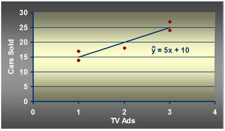
假设有一周广告数量为2,预测的汽车销售量是多少
PYTHON代码实现
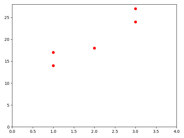
值的呈现
import numpy as np
import matplotlib.pyplot as plt
x = np.array([1, 3, 2, 1, 3])
y = np.array([14, 24, 18, 17, 27])
plt.scatter(x, y, c='r')
plt.axis([0, 4, 0, 28])
plt.show()
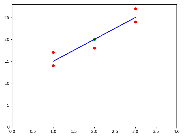
回归线的呈现
x_mean = np.mean(x)
y_mean = np.mean(y)
num = 0.0
d = 0.0
for x_i, y_i in zip(x, y):
    num += (x_i - x_mean) * (y_i - y_mean)
    d += (x_i - x_mean) ** 2
a = num/d
b = y_mean - a * x_mean
y_hat = a * x + b
plt.scatter(x, y, c='r')
plt.plot(x, y_hat, color='b')
plt.axis([0, 4, 0, 28])
plt.show()

预测值的呈现
x_predict = 2
y_predict = a * x_predict + b
plt.scatter(x_predict, y_predict, c='g')
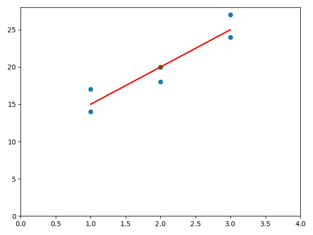
代码封装
import numpy as np
import matplotlib.pyplot as plt
class SimpleLinearRegression1:
    def __init__(self):
        # 初始化Simple Linear Regression 模型
        self.a_ = None
        self.b_ = None

    def fit(self, x_train, y_train):
        # 根据训练集x_train,y_train 训练Simple Linear Regression 模型
        assert x_train.ndim == 1, \
            "Simple Linear Regression can only solve simple feature training data"
        assert len(x_train) == len(y_train), \
            "the size of x_train must be equal to the size of y_train"
        # 求均值
        x_mean = x_train.mean()
        y_mean = y_train.mean()
        # 分子
        num = 0.0
        # 分母
        d = 0.0
        # 计算分子分母
        for x_i, y_i in zip(x_train, y_train):
            num += (x_i - x_mean) * (y_i - y_mean)
            d += (x_i - x_mean) ** 2
        # 计算参数a和b
        self.a_ = num / d
        self.b_ = y_mean - self.a_ * x_mean
        return self

    def predict(self, x_predict):
        # 给定待预测集x_predict,返回x_predict对应的预测结果值
        assert x_predict.ndim == 1, \
            "Simple Linear Regression can only solve simple feature training data"
        assert self.a_ is not None and self.b_ is not None, \
            "must fit before predict!"
        return np.array([self._predict(x) for x in x_predict])

    def _predict(self, x_single):
        # 给定单个待预测数据x_single,返回x_single对应的预测结果值
        return self.a_ * x_single + self.b_

    def __repr__(self):
        return "SimpleLinearRegression1()"

x = np.array([1, 3, 2, 1, 3])
y = np.array([14, 24, 18, 17, 27])
reg1 = SimpleLinearRegression1()
reg1.fit(x, y)
x_predict = 2
# x_predict = 2
y_predict = reg1.a_ * x_predict + reg1.b_
plt.scatter(x_predict, y_predict, c='g')
# reg1.predict(np.array([x_predict]))#单值预测
# print(reg1.a_)
# print(reg1.b_)
y_hat1 = reg1.predict(x)  # 产生多个预测值
plt.scatter(x, y)
plt.plot(x, y_hat1, color='r')
plt.axis([0, 4, 0, 28])
plt.show()
向量化
使用向量的点乘方式可以实现乘积累加求和的效果
$a=\frac{\sum_{i=1}^{m}(x^{i}-\overline{x})(y^{i}-\overline{y})}{\sum_{i=1}^{m}(x^{i}-\overline{x})^{2}}$
$\sum_{i=1}^{m}w^{i}\cdot v^{i}$
$w=(w^{1},w^{2},...,w^{m})$
$v=(v^{1},v^{2},...,v^{m})$
def fit(self, x_train, y_train):
    #根据训练数据集x_train,y_train训练Simple Linear Regression模型
    assert x_train.ndim == 1, \
        "Simple Linear Regressor can only solve single feature training data."
    assert len(x_train) == len(y_train), \
        "the size of x_train must be equal to the size of y_train"
    x_mean = np.mean(x_train)
    y_mean = np.mean(y_train)
    self.a_ = (x_train - x_mean).dot(y_train - y_mean) / (x_train - x_mean).dot(x_train - x_mean)
    self.b_ = y_mean - self.a_ * x_mean
    return self
衡量线性回归算法的指标
R Squared
$R^{2}=1-\frac{\sum (\widehat{y}^{i}-y^{i})^{2}}{\sum (\overline{y}-y^{i})^{2}}=1-\frac{\frac{\sum_{i=1}^{m}(\widehat{y}^{i}-y^{i})^{2}}{m}}{\frac{\sum_{i=1}^{m}(\overline{y}-y^{i})^{2}}{m}}=1-\frac{MSE(\widehat{y},y)}{Var(y)}$
代码实现
scikit-learn中的 r2_score
from sklearn.metrics import r2_score
s = r2_score(y_test, y_predict)
print(s)
R Squared 的意义
- $\sum (\widehat{y}^{i}-y^{i})^{2}$:使用我们的模型预测产生的错误
- $\sum (\overline{y}-y^{i})^{2}$:使用 $y=\overline{y}$ 预测产生的错误
- $R^{2}<=1$
- $R^{2}$ 越大越好,当我们的预测模型不犯任何错误时,$R^{2}$ 得到最大值1
- 当我们的模型等于基准模型时,$R^{2}=0$
- 如果 $R^{2}<0$ ,则我们的数据不存在线性关系
多元线性回归
在回归分析中,如果有两个或两个以上的自变量,就称为多元回归。事实上,一种现象常常是与多个因素相联系的,由多个自变量的最优组合共同来预测或估计因变量,比只用一个自变量进行预测或估计更有效,更符合实际。因此多元线性回归比一元线性回归的实用意义更大。
多元线性回归方程
$y=\theta _{0}+\theta _{1}x_{1}+\theta _{2}x_{2}+\cdots +\theta _{n}x_{n}$
$\theta _{0}$ :常数项
$\theta _{1}$, $\theta _{2}$,...,$\theta _{n}$ 称为 $y$ 对应于$x_{1}$, $x_{2}$,..., $x_{n}$ 的偏回归系数
$\widehat{y}^{(i)}=\theta _{0}+\theta _{1}x_{1}^{(i)}+\theta _{2}x_{2}^{(i)}+\cdots +\theta _{n}x_{n}^{(i)}$
目标:找到 $\theta _{0}$,$\theta _{1}$,...,$\theta _{n}$,使 $\sum_{i=1}^{m}(y^{(i)}-\widehat{y}^{(i)})^{2}$ 尽可能小
多元线性回归公式推导
$\widehat{y}^{(i)}=\theta _{0}+\theta _{1}x_{1}^{(i)}+\theta _{2}x_{2}^{(i)}+\cdots +\theta _{n}x_{n}^{(i)}$ , $x_{0}^{(i)}\equiv 1$
$x^{(i)}=(x_{0}^{(i)},x_{1}^{(i)},x_{2}^{(i)},\cdots ,x_{n}^{(i)})$
$\theta =(\theta _{0},\theta _{1},\theta _{2},\cdots ,\theta _{n})^{T}$
$\widehat{y}^{(i)}=x^{(i)}\cdot \theta $
$X_{b}=\begin{pmatrix}
1& x_{1}^{(1)}& x_{2}^{(1)}& x_{n}^{(1)}& \\
1& x_{1}^{(2)}& x_{2}^{(2)}& x_{n}^{(2)}& \\
\cdots & & & \cdots & \\
1& x_{1}^{(m)}& x_{2}^{(m)}& x_{n}^{(m)}&
\end{pmatrix}$ $\theta =\begin{pmatrix}
\theta _{0}\\
\theta _{1}\\
\theta _{2}\\
\cdots \\
\theta _{n}
\end{pmatrix}$
$\widehat{y}=X_{b}\cdot \theta $
使 $\sum_{i=1}^{m}(y^{(i)}-\widehat{y}^{(i)})^{2}$ 尽可能小
使 $(y-X_{b}\cdot \theta )^{T}(y-X_{b}\cdot \theta )$ 尽可能小
$\theta =(X_{b}^{T}X_{b})^{-1}X_{b}^{T}y$

 浙公网安备 33010602011771号