pandas百题笔记
Pandas百题笔记
1.导入 Pandas:
import pandas as pd
2.查看 Pandas 版本信息:
print(pd.__version__) ==>1.0.1
Pandas 的数据结构:Pandas 主要有 Series(一维数组),DataFrame(二维数组),Panel(三维数组),Panel4D(四维数组),PanelND(更多维数组)等数据结构。其中 Series 和 DataFrame 应用的最为广泛。
#Series 是一维带标签的数组,它可以包含任何数据类型。包括整数,字符串,浮点数,Python 对象等。Series 可以通过标签来定位。 #DataFrame 是二维的带标签的数据结构。我们可以通过标签来定位数据。这是 NumPy 所没有的。
创建 Series 数据类型
创建 Series 语法:s = pd.Series(data, index=index),可以通过多种方式进行创建,以下介绍了 3 个常用方法。
3.从列表创建 Series:
arr = [0, 1, 2, 3, 4]
s1 = pd.Series(arr)  # 如果不指定索引,则默认从 0 开始
s1
==>
0    0
1    1
2    2
3    3
4    4
dtype: int64
4.从 Ndarray 创建 Series:
import numpy as np

n = np.random.randn(5)  # 创建一个随机 Ndarray 数组

index = ['a', 'b', 'c', 'd', 'e']
s2 = pd.Series(n, index=index)
s2
==>
a   -0.766282
b    0.134975
c    0.175090
d    0.298047
e    0.171916
dtype: float64
5.从字典创建 Series:
d = {'a': 1, 'b': 2, 'c': 3, 'd': 4, 'e': 5}  # 定义示例字典
s3 = pd.Series(d)
s3
==>
a    1
b    2
c    3
d    4
e    5
dtype: int64
Series 基本操作
6.修改 Series 索引:
print(s1)  # 以 s1 为例

s1.index = ['A', 'B', 'C', 'D', 'E']  # 修改后的索引
s1
==>
0    0
1    1
2    2
3    3
4    4
dtype: int64
A    0
B    1
C    2
D    3
E    4
dtype: int64
7.Series 纵向拼接:
s4 = s3.append(s1)  # 将 s1 拼接到 s3
s4
==>
a    1
b    2
c    3
d    4
e    5
A    0
B    1
C    2
D    3
E    4
dtype: int64
8.Series 按指定索引删除元素:
print(s4)
s4 = s4.drop('e')  # 删除索引为 e 的值
s4
==>
a    1
b    2
c    3
d    4
e    5
A    0
B    1
C    2
D    3
E    4
dtype: int64
a    1
b    2
c    3
d    4
A    0
B    1
C    2
D    3
E    4
dtype: int64
9.Series 修改指定索引元素:
s4['A'] = 6  # 修改索引为 A 的值 = 6
s4
==>
a    1
b    2
c    3
d    4
A    6
B    1
C    2
D    3
E    4
dtype: int64
10.Series 按指定索引查找元素:
s4['B']
==>  1
11.Series 切片操作:
例如对s4的前 3 个数据访问
s4[:3]
==>
a    1
b    2
c    3
dtype: int64
Series 运算
12.Series 加法运算:
Series 的加法运算是按照索引计算,如果索引不同则填充为 NaN(空值)。
s4.add(s3)
==>
A    NaN
B    NaN
C    NaN
D    NaN
E    NaN
a    2.0
b    4.0
c    6.0
d    8.0
e    NaN
dtype: float64
13.Series 减法运算:
Series的减法运算是按照索引对应计算,如果不同则填充为 NaN(空值)。
s4.sub(s3)
==>
A    NaN
B    NaN
C    NaN
D    NaN
E    NaN
a    0.0
b    0.0
c    0.0
d    0.0
e    NaN
dtype: float64
14.Series 乘法运算:
Series 的乘法运算是按照索引对应计算,如果索引不同则填充为 NaN(空值)。
s4.mul(s3)
==>
A     NaN
B     NaN
C     NaN
D     NaN
E     NaN
a     1.0
b     4.0
c     9.0
d    16.0
e     NaN
dtype: float64
15.Series 除法运算:
Series 的除法运算是按照索引对应计算,如果索引不同则填充为 NaN(空值)。
s4.div(s3)
==>
A    NaN
B    NaN
C    NaN
D    NaN
E    NaN
a    1.0
b    1.0
c    1.0
d    1.0
e    NaN
dtype: float64
16.Series 求中位数:
s4.median() ==> 3.0
17.Series 求和:
s4.sum() ==> 26
18.Series 求最大值:
s4.max() ==> 6
19.Series 求最小值:
s4.min() ==> 1
创建 DataFrame 数据类型
与 Sereis 不同,DataFrame 可以存在多列数据。一般情况下,DataFrame 也更加常用。
20.通过 NumPy 数组创建 DataFrame:
dates = pd.date_range('today', periods=6)  # 定义时间序列作为 index
num_arr = np.random.randn(6, 4)  # 传入 numpy 随机数组
columns = ['A', 'B', 'C', 'D']  # 将列表作为列名
df1 = pd.DataFrame(num_arr, index=dates, columns=columns)
df1
==>
                                   A         B         C         D
2020-07-05 13:58:34.723797 -0.820141  0.205872 -0.928024 -1.828410
2020-07-06 13:58:34.723797  0.750014 -0.340494  1.190786 -0.204266
2020-07-07 13:58:34.723797 -2.062106 -1.520711  1.414341  1.057326
2020-07-08 13:58:34.723797 -0.821653  0.564271 -1.274913  2.340385
2020-07-09 13:58:34.723797 -1.936687  0.447897 -0.108420  0.133166
2020-07-10 13:58:34.723797  0.707222 -1.251812 -0.235982  0.340147
21.通过字典数组创建 DataFrame:
data = {'animal': ['cat', 'cat', 'snake', 'dog', 'dog', 'cat', 'snake', 'cat', 'dog', 'dog'],
        'age': [2.5, 3, 0.5, np.nan, 5, 2, 4.5, np.nan, 7, 3],
        'visits': [1, 3, 2, 3, 2, 3, 1, 1, 2, 1],
        'priority': ['yes', 'yes', 'no', 'yes', 'no', 'no', 'no', 'yes', 'no', 'no']}

labels = ['a', 'b', 'c', 'd', 'e', 'f', 'g', 'h', 'i', 'j']
df2 = pd.DataFrame(data, index=labels)
df2
==>
  animal  age  visits priority
a    cat  2.5       1      yes
b    cat  3.0       3      yes
c  snake  0.5       2       no
d    dog  NaN       3      yes
e    dog  5.0       2       no
f    cat  2.0       3       no
g  snake  4.5       1       no
h    cat  NaN       1      yes
i    dog  7.0       2       no
j    dog  3.0       1       no
#字典中的键值直接变为列名
22.查看 DataFrame 的数据类型:
df2.dtypes
==>
animal       object
age         float64
visits        int64
priority     object
dtype: object
DataFrame 基本操作
23.预览 DataFrame 的前 5 行数据:
此方法对快速了解陌生数据集结构十分有用。
df2.head()  # 默认为显示 5 行,可根据需要在括号中填入希望预览的行数
==>
    animal  age    visits priority
a    cat    2.5       1      yes
b    cat    3.0       3      yes
c  snake    0.5       2       no
d    dog    NaN       3      yes
e    dog    5.0       2       no
24.查看 DataFrame 的后 3 行数据:
df2.tail(3)
==>
    animal  age  visits priority
h    cat  NaN       1      yes
i    dog  7.0       2       no
j    dog  3.0       1       no
25.查看 DataFrame 的索引:
df2.index
==>  Index(['a', 'b', 'c', 'd', 'e', 'f', 'g', 'h', 'i', 'j'], dtype='object')
26.查看 DataFrame 的列名:
df2.columns
==>Index(['animal', 'age', 'visits', 'priority'], dtype='object')
27.查看 DataFrame 的数值:
df2.values
==>
array([['cat', 2.5, 1, 'yes'],
       ['cat', 3.0, 3, 'yes'],
       ['snake', 0.5, 2, 'no'],
       ['dog', nan, 3, 'yes'],
       ['dog', 5.0, 2, 'no'],
       ['cat', 2.0, 3, 'no'],
       ['snake', 4.5, 1, 'no'],
       ['cat', nan, 1, 'yes'],
       ['dog', 7.0, 2, 'no'],
       ['dog', 3.0, 1, 'no']], dtype=object)
28.查看 DataFrame 的统计数据:
df2.describe()
==>
            age     visits
count  8.000000  10.000000
mean   3.437500   1.900000
std    2.007797   0.875595
min    0.500000   1.000000
25%    2.375000   1.000000
50%    3.000000   2.000000
75%    4.625000   2.750000
max    7.000000   3.000000
29.DataFrame 转置操作:
   df2.T
    ==>
            a    b      c    d    e    f      g    h    i    j
    animal    cat  cat  snake  dog  dog  cat  snake  cat  dog  dog
    age       2.5    3    0.5  NaN    5    2    4.5  NaN    7    3
    visits      1    3      2    3    2    3      1    1    2    1
    priority  yes  yes     no  yes   no   no     no  yes   no   no
30.对 DataFrame 进行按列排序:
df2.sort_values(by='age')  # 按 age 升序排列
    ==>
      animal  age  visits priority
    c  snake  0.5       2       no
    f    cat  2.0       3       no
    a    cat  2.5       1      yes
    b    cat  3.0       3      yes
    j    dog  3.0       1       no
    g  snake  4.5       1       no
    e    dog  5.0       2       no
    i    dog  7.0       2       no
    d    dog  NaN       3      yes
    h    cat  NaN       1      yes
31.对 DataFrame 数据切片:
df2[1:3]
==>
    animal  age  visits priority
b    cat  3.0       3      yes
c  snake  0.5       2       no
32.对 DataFrame 通过标签查询(单列):
df2['age']
==>
a    2.5
b    3.0
c    0.5
d    NaN
e    5.0
f    2.0
g    4.5
h    NaN
i    7.0
j    3.0
Name: age, dtype: float64

df2.age  # 等价于 df2['age']
33.对 DataFrame 通过标签查询(多列):
df2[['age', 'animal']]  # 传入一个列名组成的列表
==>
   age   animal
a  2.5    cat
b  3.0    cat
c  0.5  snake
d  NaN    dog
e  5.0    dog
f  2.0    cat
g  4.5  snake
h  NaN    cat
i  7.0    dog
j  3.0    dog
34.对 DataFrame 通过位置查询:
df2.iloc[1:3]  # 查询 2,3 行
==>
    animal  age  visits priority
b    cat  3.0       3      yes
c  snake  0.5       2       no
35.DataFrame 副本拷贝:
生成 DataFrame 副本,方便数据集被多个不同流程使用
df3 = df2.copy()
df3
==>
  animal  age  visits priority
a    cat  2.5       1      yes
b    cat  3.0       3      yes
c  snake  0.5       2       no
d    dog  NaN       3      yes
e    dog  5.0       2       no
f    cat  2.0       3       no
g  snake  4.5       1       no
h    cat  NaN       1      yes
i    dog  7.0       2       no
j    dog  3.0       1       no
36.判断 DataFrame 元素是否为空:
df3.isnull()  # 如果为空则返回为 True
==>
      animal    age  visits  priority
a   False  False   False     False
b   False  False   False     False
c   False  False   False     False
d   False   True   False     False
e   False  False   False     False
f   False  False   False     False
g   False  False   False     False
h   False   True   False     False
i   False  False   False     False
j   False  False   False     False
37.添加列数据:
num = pd.Series([0, 1, 2, 3, 4, 5, 6, 7, 8, 9], index=df3.index)

df3['No.'] = num  # 添加以 'No.' 为列名的新数据列
df3
==>
  animal  age  visits priority  No.
a    cat  2.5       1      yes    0
b    cat  3.0       3      yes    1
c  snake  0.5       2       no    2
d    dog  NaN       3      yes    3
e    dog  5.0       2       no    4
f    cat  2.0       3       no    5
g  snake  4.5       1       no    6
h    cat  NaN       1      yes    7
i    dog  7.0       2       no    8
j    dog  3.0       1       no    9
38.根据 DataFrame 的下标值进行更改:
修改第 2 行与第 2 列对应的值 3.0 → 2.0
df3.iat[1, 1] = 2  # 索引序号从 0 开始,这里为 1, 1
df3
==>
  animal  age  visits priority  No.
a    cat  2.5       1      yes    0
b    cat  2.0       3      yes    1
c  snake  0.5       2       no    2
d    dog  NaN       3      yes    3
e    dog  5.0       2       no    4
f    cat  2.0       3       no    5
g  snake  4.5       1       no    6
h    cat  NaN       1      yes    7
i    dog  7.0       2       no    8
j    dog  3.0       1       no    9
39.根据 DataFrame 的标签对数据进行修改:
df3.loc['f', 'age'] = 1.5
df3
==>
    animal  age  visits priority  No.
a    cat  2.5       1      yes    0
b    cat  2.0       3      yes    1
c  snake  0.5       2       no    2
d    dog  NaN       3      yes    3
e    dog  5.0       2       no    4
f    cat  1.5       3       no    5
g  snake  4.5       1       no    6
h    cat  NaN       1      yes    7
i    dog  7.0       2       no    8
j    dog  3.0       1       no    9
40.DataFrame 求平均值操作:
df3.mean()
==>
age       3.25
visits    1.90
No.       4.50
dtype: float64
41.对 DataFrame 中任意列做求和操作:
df3['visits'].sum()
==> 19
字符串操作
42.将字符串转化为小写字母:
string = pd.Series(['A', 'B', 'C', 'Aaba', 'Baca',
                    np.nan, 'CABA', 'dog', 'cat'])
print(string)
string.str.lower()
==>
0       A
1       B
2       C
3    Aaba
4    Baca
5     NaN
6    CABA
7     dog
8     cat
dtype: object
0       a
1       b
2       c
3    aaba
4    baca
5     NaN
6    caba
7     dog
8     cat
dtype: object
43.将字符串转化为大写字母:
string.str.upper()
==>
0       A
1       B
2       C
3    AABA
4    BACA
5     NaN
6    CABA
7     DOG
8     CAT
dtype: object
DataFrame 缺失值操作
44.对缺失值进行填充:
df4 = df3.copy()
print(df4)
df4.fillna(value=3)
==>
    animal  age  visits priority  No.
a    cat  2.5       1      yes    0
b    cat  2.0       3      yes    1
c  snake  0.5       2       no    2
d    dog  NaN       3      yes    3
e    dog  5.0       2       no    4
f    cat  1.5       3       no    5
g  snake  4.5       1       no    6
h    cat  NaN       1      yes    7
i    dog  7.0       2       no    8
j    dog  3.0       1       no    9

  animal  age  visits priority  No.
a    cat  2.5       1      yes    0
b    cat  2.0       3      yes    1
c  snake  0.5       2       no    2
d    dog  3.0       3      yes    3
e    dog  5.0       2       no    4
f    cat  1.5       3       no    5
g  snake  4.5       1       no    6
h    cat  3.0       1      yes    7
i    dog  7.0       2       no    8
j    dog  3.0       1       no    9
45.删除存在缺失值的行:
df5 = df3.copy()
print(df5)
df5.dropna(how='any')  # 任何存在 NaN 的行都将被删除
==>
    animal  age  visits priority  No.
a    cat  2.5       1      yes    0
b    cat  2.0       3      yes    1
c  snake  0.5       2       no    2
d    dog  NaN       3      yes    3
e    dog  5.0       2       no    4
f    cat  1.5       3       no    5
g  snake  4.5       1       no    6
h    cat  NaN       1      yes    7
i    dog  7.0       2       no    8
j    dog  3.0       1       no    9

  animal  age  visits priority  No.
a    cat  2.5       1      yes    0
b    cat  2.0       3      yes    1
c  snake  0.5       2       no    2
e    dog  5.0       2       no    4
f    cat  1.5       3       no    5
g  snake  4.5       1       no    6
i    dog  7.0       2       no    8
j    dog  3.0       1       no    9
46.DataFrame 按指定列对齐:
left = pd.DataFrame({'key': ['foo1', 'foo2'], 'one': [1, 2]})
right = pd.DataFrame({'key': ['foo2', 'foo3'], 'two': [4, 5]})

print(left)
print(right)
按照 key 列对齐连接,只存在 foo2 相同,所以最后变成一行
pd.merge(left, right, on='key')
==>
key one
0 foo1 1
1 foo2 2
key two
0 foo2 4
1 foo3 5
key one two
0 foo2 2 4
DataFrame 文件操作
47.CSV 文件写入:
df3.to_csv('animal.csv')
print("写入成功.")
==>  写入成功.
48.CSV 文件读取:
df_animal = pd.read_csv('animal.csv')
df_animal
==>
    Unnamed: 0 animal  age  visits priority  No.
0          a    cat  2.5       1      yes    0
1          b    cat  2.0       3      yes    1
2          c  snake  0.5       2       no    2
3          d    dog  NaN       3      yes    3
4          e    dog  5.0       2       no    4
5          f    cat  1.5       3       no    5
6          g  snake  4.5       1       no    6
7          h    cat  NaN       1      yes    7
8          i    dog  7.0       2       no    8
9          j    dog  3.0       1       no    9
49.Excel 写入操作:
df3.to_excel('animal.xlsx', sheet_name='Sheet1')
print("写入成功.")
==>  写入成功.
50.Excel 读取操作:
pd.read_excel('animal.xlsx', 'Sheet1', index_col=None, na_values=['NA'])
==>
    Unnamed: 0 animal  age  visits priority  No.
0          a    cat  2.5       1      yes    0
1          b    cat  2.0       3      yes    1
2          c  snake  0.5       2       no    2
3          d    dog  NaN       3      yes    3
4          e    dog  5.0       2       no    4
5          f    cat  1.5       3       no    5
6          g  snake  4.5       1       no    6
7          h    cat  NaN       1      yes    7
8          i    dog  7.0       2       no    8
9          j    dog  3.0       1       no    9
进阶部分
时间序列索引
51.建立一个以 2018 年每一天为索引,值为随机数的 Series:
dti = pd.date_range(start='2018-01-01', end='2018-12-31', freq='D')
s = pd.Series(np.random.rand(len(dti)), index=dti)
s
==>
2018-01-01    0.441330
2018-01-02    0.182571
2018-01-03    0.141348
2018-01-04    0.604700
2018-01-05    0.300351
                ...
2018-12-27    0.499318
2018-12-28    0.530867
2018-12-29    0.183895
2018-12-30    0.163899
2018-12-31    0.173812
Freq: D, Length: 365, dtype: float64
52.统计s 中每一个周三对应值的和:
周一从 0 开始
s[s.index.weekday == 2].sum()
==>  22.592391213957054
53.统计s中每个月值的平均值:
s.resample('M').mean()
==>
2018-01-31    0.441100
2018-02-28    0.506476
2018-03-31    0.501672
2018-04-30    0.510073
2018-05-31    0.416773
2018-06-30    0.525039
2018-07-31    0.433221
2018-08-31    0.472530
2018-09-30    0.388529
2018-10-31    0.550011
2018-11-30    0.486513
2018-12-31    0.443012
Freq: M, dtype: float64
54.将 Series 中的时间进行转换(秒转分钟):
s = pd.date_range('today', periods=100, freq='S')

ts = pd.Series(np.random.randint(0, 500, len(s)), index=s)

ts.resample('Min').sum()
==>
2020-07-05 14:48:00    15836
2020-07-05 14:49:00     9298
Freq: T, dtype: int64
55.UTC 世界时间标准:
s = pd.date_range('today', periods=1, freq='D')  # 获取当前时间
ts = pd.Series(np.random.randn(len(s)), s)  # 随机数值
ts_utc = ts.tz_localize('UTC')  # 转换为 UTC 时间
ts_utc
==>
2020-07-05 14:48:38.609382+00:00   -0.348899
Freq: D, dtype: float64
56.转换为上海所在时区:
ts_utc.tz_convert('Asia/Shanghai')
==>
2020-07-05 22:48:38.609382+08:00   -0.348899
Freq: D, dtype: float64
57.不同时间表示方式的转换:
rng = pd.date_range('1/1/2018', periods=5, freq='M')
ts = pd.Series(np.random.randn(len(rng)), index=rng)
print(ts)
ps = ts.to_period()
print(ps)
ps.to_timestamp()
==>
2018-01-31    0.621688
2018-02-28   -1.937715
2018-03-31    0.081314
2018-04-30   -1.308769
2018-05-31   -0.075345
Freq: M, dtype: float64
2018-01    0.621688
2018-02   -1.937715
2018-03    0.081314
2018-04   -1.308769
2018-05   -0.075345
Freq: M, dtype: float64
2018-01-01    0.621688
2018-02-01   -1.937715
2018-03-01    0.081314
2018-04-01   -1.308769
2018-05-01   -0.075345
Freq: MS, dtype: float64
Series 多重索引
58.创建多重索引 Series:
构建一个 letters = ['A', 'B', 'C'] 和 numbers = list(range(10))为索引,值为随机数的多重索引 Series。
letters = ['A', 'B', 'C']
numbers = list(range(10))

mi = pd.MultiIndex.from_product([letters, numbers])  # 设置多重索引
s = pd.Series(np.random.rand(30), index=mi)  # 随机数
s
==>
A  0    0.698046
   1    0.380276
   2    0.873395
   3    0.628864
   4    0.528025
   5    0.677856
   6    0.194495
   7    0.164484
   8    0.018238
   9    0.747468
B  0    0.623616
   1    0.560504
   2    0.731296
   3    0.760307
   4    0.807663
   5    0.347980
   6    0.005892
   7    0.807262
   8    0.650353
   9    0.803976
C  0    0.387503
   1    0.943305
   2    0.215817
   3    0.128086
   4    0.252103
   5    0.048908
   6    0.779633
   7    0.825234
   8    0.624257
   9    0.263373
dtype: float64
59.多重索引 Series 查询:
查询索引为 1,3,6 的值
s.loc[:, [1, 3, 6]]
==>
A  1    0.380276
   3    0.628864
   6    0.194495
B  1    0.560504
   3    0.760307
   6    0.005892
C  1    0.943305
   3    0.128086
   6    0.779633
dtype: float64
60.多重索引 Series 切片:
s.loc[pd.IndexSlice[:'B', 5:]]
==>
A  5    0.677856
      6    0.194495
      7    0.164484
      8    0.018238
      9    0.747468
B  5    0.347980
      6    0.005892
      7    0.807262
      8    0.650353
      9    0.803976
dtype: float64
DataFrame 多重索引
61.根据多重索引创建 DataFrame:
创建一个以 letters = ['A', 'B'] 和 numbers = list(range(6))为索引,值为随机数据的多重索引 DataFrame。
frame = pd.DataFrame(np.arange(12).reshape(6, 2),
                     index=[list('AAABBB'), list('123123')],
                     columns=['hello', 'shiyanlou'])
frame
==>
     hello  shiyanlou
A 1      0          1
    2      2          3
    3      4          5
B 1      6          7
    2      8          9
    3     10         11
62.多重索引设置列名称:
frame.index.names = ['first', 'second']
frame
==>
                 hello    shiyanlou
first second
A       1           0          1
        2           2          3
        3           4          5
B       1           6          7
        2           8          9
        3          10         11
63.DataFrame 多重索引分组求和:
frame.groupby('first').sum()
==>
       hello  shiyanlou
first
A          6          9
B         24         27
64.DataFrame 行列名称转换:
print(frame)
frame.stack()
==>
              hello  shiyanlou
first second
A     1           0          1
      2           2          3
      3           4          5
B     1           6          7
      2           8          9
      3          10         11
first  second
A      1       hello         0
               shiyanlou     1
       2       hello         2
               shiyanlou     3
       3       hello         4
               shiyanlou     5
B      1       hello         6
               shiyanlou     7
       2       hello         8
               shiyanlou     9
       3       hello        10
               shiyanlou    11
dtype: int64
65.DataFrame 索引转换:
print(frame)
frame.unstack()
==>
              hello  shiyanlou
first second
A     1           0          1
      2           2          3
      3           4          5
B     1           6          7
      2           8          9
      3          10         11
       hello        shiyanlou
second     1  2   3         1  2   3
first
A          0  2   4         1  3   5
B          6  8  10         7  9  11
66.DataFrame 条件查找:
示例数据
data = {'animal': ['cat', 'cat', 'snake', 'dog', 'dog', 'cat', 'snake', 'cat', 'dog', 'dog'],
        'age': [2.5, 3, 0.5, np.nan, 5, 2, 4.5, np.nan, 7, 3],
        'visits': [1, 3, 2, 3, 2, 3, 1, 1, 2, 1],
        'priority': ['yes', 'yes', 'no', 'yes', 'no', 'no', 'no', 'yes', 'no', 'no']}

labels = ['a', 'b', 'c', 'd', 'e', 'f', 'g', 'h', 'i', 'j']
df = pd.DataFrame(data, index=labels)
查找 age 大于 3 的全部信息
df[df['age'] > 3]
==>
  animal  age  visits priority
e    dog  5.0       2       no
g  snake  4.5       1       no
i    dog  7.0       2       no
67.根据行列索引切片:
df.iloc[2:4, 1:3]
==>
      age  visits
c  0.5       2
d  NaN       3
68.DataFrame 多重条件查询:
查找 age<3 且为 cat 的全部数据。
df = pd.DataFrame(data, index=labels)

df[(df['animal'] == 'cat') & (df['age'] < 3)]
==>
  animal  age  visits priority
a    cat  2.5       1      yes
f    cat  2.0       3       no
69.DataFrame 按关键字查询:
df3[df3['animal'].isin(['cat', 'dog'])]
==>
    animal  age  visits priority  No.
a    cat  2.5       1      yes    0
b    cat  2.0       3      yes    1
d    dog  NaN       3      yes    3
e    dog  5.0       2       no    4
f    cat  1.5       3       no    5
h    cat  NaN       1      yes    7
i    dog  7.0       2       no    8
j    dog  3.0       1       no    9
70.DataFrame 按标签及列名查询:
df.loc[df2.index[[3, 4, 8]], ['animal', 'age']]
==>
    animal  age
d    dog  NaN
e    dog  5.0
i    dog  7.0
71.DataFrame 多条件排序:
按照 age 降序,visits 升序排列
df.sort_values(by=['age', 'visits'], ascending=[False, True])
==>
    animal  age  visits priority
i    dog  7.0       2       no
e    dog  5.0       2       no
g  snake  4.5       1       no
j    dog  3.0       1       no
b    cat  3.0       3      yes
a    cat  2.5       1      yes
f    cat  2.0       3       no
c  snake  0.5       2       no
h    cat  NaN       1      yes
d    dog  NaN       3      yes
72.DataFrame 多值替换:
将 priority 列的 yes 值替换为 True,no 值替换为 False。
df['priority'].map({'yes': True, 'no': False})
==>
a     True
b     True
c    False
d     True
e    False
f    False
g    False
h     True
i    False
j    False
Name: priority, dtype: bool
73.DataFrame 分组求和:
df4.groupby('animal').sum()
==>
         age  visits  No.
animal
cat      6.0       8   13
dog     15.0       8   24
snake    5.0       3    8
74.使用列表拼接多个 DataFrame:
temp_df1 = pd.DataFrame(np.random.randn(5, 4)) # 生成由随机数组成的 DataFrame 1
temp_df2 = pd.DataFrame(np.random.randn(5, 4)) # 生成由随机数组成的 DataFrame 2
temp_df3 = pd.DataFrame(np.random.randn(5, 4)) # 生成由随机数组成的 DataFrame 3
print(temp_df1)
print(temp_df2)
print(temp_df3)
pieces = [temp_df1, temp_df2, temp_df3]
pd.concat(pieces)
==>
0 1 2 3
0 1.061349 0.927805 -0.270724 0.232218
1 -2.049875 -0.896899 -0.738298 0.547709
2 0.084709 -1.801844 0.610220 -1.304246
3 1.384591 0.872657 -0.829547 -0.332316
4 -0.255004 2.177881 0.615079 0.767592
0 1 2 3
0 0.009016 1.181569 -1.403829 -0.745604
1 -0.270313 -0.258377 -1.067346 1.465726
2 -1.619676 -0.324374 -0.433600 0.211323
3 0.163223 0.144191 0.717129 -0.555298
4 -0.718321 1.688866 -0.607994 1.731248
0 1 2 3
0 -1.178622 0.415409 0.496004 1.368869
1 0.724433 -0.262059 0.514689 -1.666051
2 -0.325606 0.013015 1.010961 2.075196
3 2.212960 -0.132432 -1.603347 -1.182487
4 0.102536 1.384535 0.411434 -0.175592
0 1 2 3
0 1.061349 0.927805 -0.270724 0.232218
1 -2.049875 -0.896899 -0.738298 0.547709
2 0.084709 -1.801844 0.610220 -1.304246
3 1.384591 0.872657 -0.829547 -0.332316
4 -0.255004 2.177881 0.615079 0.767592
0 0.009016 1.181569 -1.403829 -0.745604
1 -0.270313 -0.258377 -1.067346 1.465726
2 -1.619676 -0.324374 -0.433600 0.211323
3 0.163223 0.144191 0.717129 -0.555298
4 -0.718321 1.688866 -0.607994 1.731248
0 -1.178622 0.415409 0.496004 1.368869
1 0.724433 -0.262059 0.514689 -1.666051
2 -0.325606 0.013015 1.010961 2.075196
3 2.212960 -0.132432 -1.603347 -1.182487
4 0.102536 1.384535 0.411434 -0.175592
75.找出 DataFrame 表中和最小的列:
df = pd.DataFrame(np.random.random(size=(5, 10)), columns=list('abcdefghij'))
print(df)
df.sum().idxmin() # idxmax(), idxmin() 为 Series 函数返回最大最小值的索引值
==>
a b c d e f g \
0 0.931149 0.641776 0.758608 0.630512 0.170375 0.211306 0.973363
1 0.730186 0.682949 0.554609 0.356089 0.399012 0.939087 0.908047
2 0.261405 0.434525 0.490395 0.368307 0.832568 0.571115 0.936016
3 0.161993 0.132176 0.852158 0.140710 0.165902 0.564976 0.656718
4 0.810233 0.385639 0.127849 0.166585 0.302643 0.947498 0.164274
h i j
0 0.223378 0.115285 0.161207
1 0.765946 0.206518 0.951096
2 0.891956 0.430530 0.045640
3 0.955571 0.962989 0.123037
4 0.391810 0.696404 0.561719
'd'
76.DataFrame 中每个元素减去每一行的平均值:
df = pd.DataFrame(np.random.random(size=(5, 3)))
print(df)
df.sub(df.mean(axis=1), axis=0)
==>
0 1 2
0 0.028539 0.555065 0.166588
1 0.781335 0.086089 0.616780
2 0.022462 0.047383 0.476410
3 0.796853 0.850955 0.765398
4 0.208298 0.858031 0.264920
0 1 2
0 -0.221525 0.305001 -0.083476
1 0.286600 -0.408646 0.122046
2 -0.159623 -0.134702 0.294325
3 -0.007549 0.046553 -0.039004
4 -0.235452 0.414281 -0.178830
77.DataFrame 分组,并得到每一组中最大三个数之和:
df = pd.DataFrame({'A': list('aaabbcaabcccbbc'),
                   'B': [12, 345, 3, 1, 45, 14, 4, 52, 54, 23, 235, 21, 57, 3, 87]})
print(df)
df.groupby('A')['B'].nlargest(3).sum(level=0)
==>
    A    B
0   a   12
1   a  345
2   a    3
3   b    1
4   b   45
5   c   14
6   a    4
7   a   52
8   b   54
9   c   23
10  c  235
11  c   21
12  b   57
13  b    3
14  c   87
A
a    409
b    156
c    345
Name: B, dtype: int64
透视表
当分析庞大的数据时,为了更好的发掘数据特征之间的关系,且不破坏原数据,就可以利用透视表 pivot_table 进行操作。
78.透视表的创建:
新建表将 A, B, C 列作为索引进行聚合。
df = pd.DataFrame({'A': ['one', 'one', 'two', 'three'] * 3,
'B': ['A', 'B', 'C'] * 4,
'C': ['foo', 'foo', 'foo', 'bar', 'bar', 'bar'] * 2,
'D': np.random.randn(12),
'E': np.random.randn(12)})
print(df)
print(pd.pivot_table(df, index=['A', 'B']))
==>
A B C D E
0 one A foo -2.718717 1.749056
1 one B foo -0.710776 0.442023
2 two C foo -0.824951 2.244523
3 three A bar 0.300916 1.709200
4 one B bar -2.590790 0.292709
5 one C bar 0.908543 -0.598258
6 two A foo -0.521278 0.204491
7 three B foo -3.302320 -1.762640
8 one C foo -1.311013 -0.722187
9 one A bar 0.785471 -0.231635
10 two B bar -1.758329 -0.031603
11 three C bar 1.236829 1.235032
D E
A B
one A -0.966623 0.758711
B -1.650783 0.367366
C -0.201235 -0.660222
three A 0.300916 1.709200
B -3.302320 -1.762640
C 1.236829 1.235032
two A -0.521278 0.204491
B -1.758329 -0.031603
C -0.824951 2.244523
79.透视表按指定行进行聚合:
将该 DataFrame 的 D 列聚合,按照 A,B 列为索引进行聚合,聚合的方式为默认求均值。
pd.pivot_table(df, values=['D'], index=['A', 'B'])
==>
                D
A     B
one   A -0.966623
      B -1.650783
      C -0.201235
three A  0.300916
      B -3.302320
      C  1.236829
two   A -0.521278
      B -1.758329
      C -0.824951
80.透视表聚合方式定义:
上一题中 D 列聚合时,采用默认求均值的方法,若想使用更多的方式可以在 aggfunc 中实现。
pd.pivot_table(df, values=['D'], index=['A', 'B'], aggfunc=[np.sum, len])
==>
              sum  len
                D    D
A     B
one   A -1.933246  2.0
      B -3.301567  2.0
      C -0.402470  2.0
three A  0.300916  1.0
      B -3.302320  1.0
      C  1.236829  1.0
two   A -0.521278  1.0
      B -1.758329  1.0
      C -0.824951  1.0
81.透视表利用额外列进行辅助分割:
D 列按照 A,B 列进行聚合时,若关心 C 列对 D 列的影响,可以加入 columns 值进行分析。
pd.pivot_table(df, values=['D'], index=['A', 'B'],
               columns=['C'], aggfunc=np.sum)
==>
                D
C             bar       foo
A     B
one   A  0.785471 -2.718717
      B -2.590790 -0.710776
      C  0.908543 -1.311013
three A  0.300916       NaN
      B       NaN -3.302320
      C  1.236829       NaN
two   A       NaN -0.521278
      B -1.758329       NaN
      C       NaN -0.824951
82.透视表的缺省值处理:
在透视表中由于不同的聚合方式,相应缺少的组合将为缺省值,可以加入 fill_value 对缺省值处理。
pd.pivot_table(df, values=['D'], index=['A', 'B'],
               columns=['C'], aggfunc=np.sum, fill_value=0)
==>
                D
C             bar       foo
A     B
one   A  0.785471 -2.718717
      B -2.590790 -0.710776
      C  0.908543 -1.311013
three A  0.300916  0.000000
      B  0.000000 -3.302320
      C  1.236829  0.000000
two   A  0.000000 -0.521278
      B -1.758329  0.000000
      C  0.000000 -0.824951
绝对类型
在数据的形式上主要包括数量型和性质型,数量型表示着数据可数范围可变,而性质型表示范围已经确定不可改变,绝对型数据就是性质型数据的一种。
83.绝对型数据定义:
df = pd.DataFrame({"id": [1, 2, 3, 4, 5, 6], "raw_grade": [
                  'a', 'b', 'b', 'a', 'a', 'e']})
df["grade"] = df["raw_grade"].astype("category")
df
==>
      id raw_grade grade
0   1         a     a
1   2         b     b
2   3         b     b
3   4         a     a
4   5         a     a
5   6         e     e
84.对绝对型数据重命名:
df["grade"].cat.categories = ["very good", "good", "very bad"]
df
==>
      id raw_grade      grade
0   1         a  very good
1   2         b       good
2   3         b       good
3   4         a  very good
4   5         a  very good
5   6         e   very bad
85.重新排列绝对型数据并补充相应的缺省值:
df["grade"] = df["grade"].cat.set_categories(
    ["very bad", "bad", "medium", "good", "very good"])
df
==>
      id raw_grade      grade
0   1         a  very good
1   2         b       good
2   3         b       good
3   4         a  very good
4   5         a  very good
5   6         e   very bad
86.对绝对型数据进行排序:
df.sort_values(by="grade")
==>
      id raw_grade      grade
5   6         e   very bad
1   2         b       good
2   3         b       good
0   1         a  very good
3   4         a  very good
4   5         a  very good
87.对绝对型数据进行分组:
df.groupby("grade").size()
==>
grade
very bad     1
bad          0
medium       0
good         2
very good    3
dtype: int64
数据清洗
常常我们得到的数据是不符合我们最终处理的数据要求,包括许多缺省值以及坏的数据,需要我们对数据进行清洗。
88.缺失值拟合:
在FilghtNumber中有数值缺失,其中数值为按 10 增长,补充相应的缺省值使得数据完整,并让数据为 int 类型。
df = pd.DataFrame({'From_To': ['LoNDon_paris', 'MAdrid_miLAN', 'londON_StockhOlm',
                               'Budapest_PaRis', 'Brussels_londOn'],
                   'FlightNumber': [10045, np.nan, 10065, np.nan, 10085],
                   'RecentDelays': [[23, 47], [], [24, 43, 87], [13], [67, 32]],
                   'Airline': ['KLM(!)', '<Air France> (12)', '(British Airways. )',
                               '12. Air France', '"Swiss Air"']})
df['FlightNumber'] = df['FlightNumber'].interpolate().astype(int)
df
==>
            From_To  FlightNumber  RecentDelays              Airline
0      LoNDon_paris         10045      [23, 47]               KLM(!)
1      MAdrid_miLAN         10055            []    <Air France> (12)
2  londON_StockhOlm         10065  [24, 43, 87]  (British Airways. )
3    Budapest_PaRis         10075          [13]       12. Air France
4   Brussels_londOn         10085      [67, 32]          "Swiss Air"
89.数据列拆分:
其中From_to应该为两独立的两列From和To,将From_to依照_拆分为独立两列建立为一个新表。
temp = df.From_To.str.split('_', expand=True)
temp.columns = ['From', 'To']
temp
==>
       From         To
0    LoNDon      paris
1    MAdrid      miLAN
2    londON  StockhOlm
3  Budapest      PaRis
4  Brussels     londOn
90.字符标准化:
其中注意到地点的名字都不规范(如:londON应该为London)需要对数据进行标准化处理。
temp['From'] = temp['From'].str.capitalize()
temp['To'] = temp['To'].str.capitalize()
91.删除坏数据加入整理好的数据:
将最开始的 From_to 列删除,加入整理好的 From 和 to 列。
df = df.drop('From_To', axis=1)
df = df.join(temp)
print(df)
==>
      FlightNumber  RecentDelays              Airline      From         To
0         10045      [23, 47]               KLM(!)    London      Paris
1         10055            []    <Air France> (12)    Madrid      Milan
2         10065  [24, 43, 87]  (British Airways. )    London  Stockholm
3         10075          [13]       12. Air France  Budapest      Paris
4         10085      [67, 32]          "Swiss Air"  Brussels     London
92.去除多余字符:
如同 airline 列中许多数据有许多其他字符,会对后期的数据分析有较大影响,需要对这类数据进行修正。
df['Airline'] = df['Airline'].str.extract(
    '([a-zA-Z\s]+)', expand=False).str.strip()
df
==>
      FlightNumber          Airline      From         To  delay_1  delay_2  \
0         10045              KLM    London      Paris     23.0     47.0
1         10055       Air France    Madrid      Milan      NaN      NaN
2         10065  British Airways    London  Stockholm     24.0     43.0
3         10075       Air France  Budapest      Paris     13.0      NaN
4         10085        Swiss Air  Brussels     London     67.0     32.0

   delay_3
0      NaN
1      NaN
2     87.0
3      NaN
4      NaN
93.格式规范:
在 RecentDelays 中记录的方式为列表类型,由于其长度不一,这会为后期数据分析造成很大麻烦。这里将 RecentDelays 的列表拆开,取出列表中的相同位置元素作为一列,若为空值即用 NaN 代替。
delays = df['RecentDelays'].apply(pd.Series)

delays.columns = ['delay_{}'.format(n)
                  for n in range(1, len(delays.columns)+1)]

df = df.drop('RecentDelays', axis=1).join(delays)
df
==>
    FlightNumber	Airline	     From	         To	    delay_1	delay_2	delay_3
0       10045         KLM	    London          Paris     23.0    47.0    NaN
1       10055   Air France      Madrid          Milan     NaN     NaN     NaN
2       10065   British Airways London        Stockholm   24.0    43.0    87.0
3       10075   Air France      Budapest        Paris     13.0    NaN     NaN
4       10085   Swiss Air       Brussels        London    67.0    32.0    NaN
数据预处理
94.信息区间划分:
班级一部分同学的数学成绩表,如下图所示
df=pd.DataFrame({'name':['Alice','Bob','Candy','Dany','Ella','Frank','Grace','Jenny'],
                 'grades':[58,83,79,65,93,45,61,88]})
但我们更加关心的是该同学是否及格,将该数学成绩按照是否>60来进行划分。
df = pd.DataFrame({'name': ['Alice', 'Bob', 'Candy', 'Dany', 'Ella',
                            'Frank', 'Grace', 'Jenny'],
                   'grades': [58, 83, 79, 65, 93, 45, 61, 88]})


def choice(x):
    if x > 60:
        return 1
    else:
        return 0


df.grades = pd.Series(map(lambda x: choice(x), df.grades))
df
==>
    name  grades
0  Alice       0
1    Bob       1
2  Candy       1
3   Dany       1
4   Ella       1
5  Frank       0
6  Grace       1
7  Jenny       1
95.数据去重:
一个列为A的 DataFrame 数据,如下图所示
df = pd.DataFrame({'A': [1, 2, 2, 3, 4, 5, 5, 5, 6, 7, 7]})
尝试将 A 列中连续重复的数据清除。
df = pd.DataFrame({'A': [1, 2, 2, 3, 4, 5, 5, 5, 6, 7, 7]})
df.loc[df['A'].shift() != df['A']]
==>
      A
0  1
1  2
3  3
4  4
5  5
8  6
9  7
96.数据归一化:
有时候,DataFrame 中不同列之间的数据差距太大,需要对其进行归一化处理。 其中,Max-Min 归一化是简单而常见的一种方式,公式如下:
def normalization(df):
numerator = df.sub(df.min())
denominator = (df.max()).sub(df.min())
Y = numerator.div(denominator)
return Y
df = pd.DataFrame(np.random.random(size=(5, 3)))
print(df)
normalization(df)
==>
0 1 2
0 0.923325 0.925392 0.203170
1 0.770389 0.050410 0.605788
2 0.146447 0.542584 0.056240
3 0.161917 0.841527 0.547914
4 0.948175 0.814426 0.980268
0 1 2
0 0.969004 1.000000 0.159009
1 0.778247 0.000000 0.594731
2 0.000000 0.562496 0.000000
3 0.019297 0.904153 0.532098
4 1.000000 0.873179 1.000000
Pandas 绘图操作
为了更好的了解数据包含的信息,最直观的方法就是将其绘制成图。
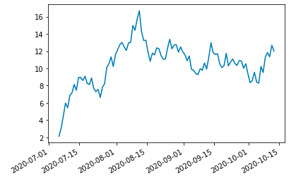
97.Series 可视化:
%matplotlib inline
ts = pd.Series(np.random.randn(100), index=pd.date_range('today', periods=100))
ts = ts.cumsum()
ts.plot()
==>输出图像:
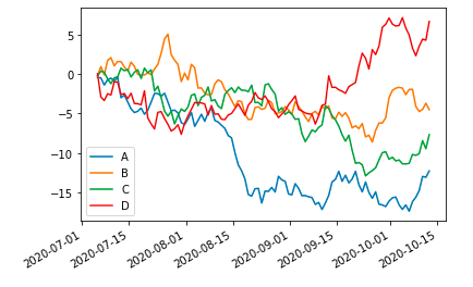
98.DataFrame 折线图:
df = pd.DataFrame(np.random.randn(100, 4), index=ts.index,
                  columns=['A', 'B', 'C', 'D'])
df = df.cumsum()
df.plot()
==>输出图像:
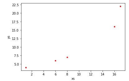
99.DataFrame 散点图:
df = pd.DataFrame({"xs": [1, 5, 2, 8, 1], "ys": [4, 2, 1, 9, 6]})
df = df.cumsum()
df.plot.scatter("xs", "ys", color='red', marker="*")
==>输出图像:
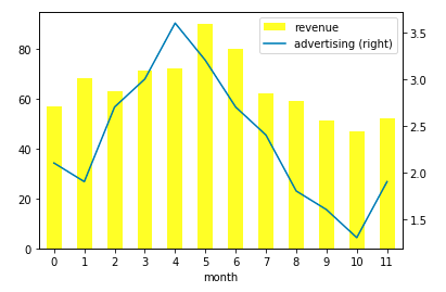
100.DataFrame 柱形图:
df = pd.DataFrame({"revenue": [57, 68, 63, 71, 72, 90, 80, 62, 59, 51, 47, 52],
                   "advertising": [2.1, 1.9, 2.7, 3.0, 3.6, 3.2, 2.7, 2.4, 1.8, 1.6, 1.3, 1.9],
                   "month": range(12)
                   })

ax = df.plot.bar("month", "revenue", color="yellow")
df.plot("month", "advertising", secondary_y=True, ax=ax)
==>输出图像:

 浙公网安备 33010602011771号