【阅读】变分自编码器 - VAE: Variational Auto-Encoder

参考：
Weng, Lilian. From Autoencoder to Beta-VAE
苏剑林. (Mar. 18, 2018). 《变分自编码器（一）：原来是这么一回事》
pytorch 实现参考

总之，VAE 本身是一个解编码的模型，我们假设观测的某个变量 \(\mathbf{x}\)（比如数字 0~9 的各种图像）受到隐变量 \(\mathbf{z}\) 的影响，那么在得到分布后，只需要采样得到一个 \(\mathbf{z}\)，我们就能生成一个 \(\mathbf{x}\)

Autocoder is invented to reconstruct high-dimensional data using a neural network model. A nice byproduct is dimension reduction: the bottleneck layer captures a compressed latent encoding. Such a low-dimensional representation can be used as en embedding vector in various applications (i.e. search), help data compression, or reveal the underlying data generative factors.

Notation

Symbol	Mean
\(\mathcal{D}\)	The dataset, \(\mathcal{D} = \{ \mathbf{x}^{(1)}, \mathbf{x}^{(2)}, \dots, \mathbf{x}^{(n)} \}\) , contains \(n\) data samples; \(\vert\mathcal{D}\vert =n\).
\(\mathbf{x}^{(i)}\)	Each data point is a vector of \(d\) dimensions, \(\mathbf{x}^{(i)} = [x^{(i)}_1, x^{(i)}_2, \dots, x^{(i)}_d]\).
\(\mathbf{x}\)	One data sample from the dataset, \(\mathbf{x} \in \mathcal{D}\).
\(\mathbf{x}'\)	The reconstructed version of \(\mathbf{x}\).
\(\tilde{\mathbf{x}}\)	The corrupted version of \(\mathbf{x}\).
\(\mathbf{z}\)	The compressed code learned in the bottleneck layer.
\(a_j^{(l)}\)	The activation function for the \(j\)-th neuron in the \(l\)-th hidden layer.
\(g_{\phi}(.)\)	The encoding function parameterized by \(\phi\).
\(f_{\theta}(.)\)	The decoding function parameterized by \(\theta\).
\(q_{\phi}(\mathbf{z}\vert\mathbf{x})\)	Estimated posterior probability function, also known as probabilistic encoder.
\(p_{\theta}(\mathbf{x}\vert\mathbf{z})\)	Likelihood of generating true data sample given the latent code, also known as probabilistic decoder.

Autoencoder

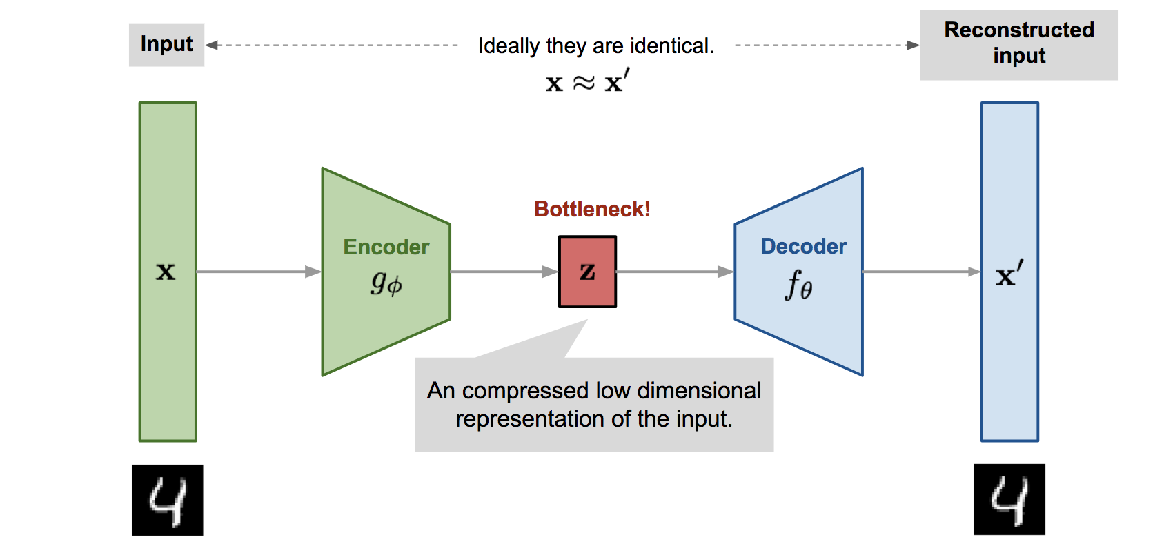
The model contains an encoder function \(g(.)\) parameterized by \(\phi\) and a decoder function \(f(.)\) parameterized by \(\theta\). The low-dimensional code learned for input \(\mathbf{x}\) in the bottleneck layer is \(\mathbf{z} = g_\phi(\mathbf{x})\) and the reconstructed input is \(\mathbf{x}' = f_\theta(g_\phi(\mathbf{x}))\).

The parameters \((\theta, \phi)\) are learned together to output a reconstructed data sample same as the original input, \(\mathbf{x} \approx f_\theta(g_\phi(\mathbf{x}))\), or in other words, to learn an identity function. A simple metric is MSE loss:

\[L_\text{AE}(\theta, \phi) = \frac{1}{n}\sum_{i=1}^n (\mathbf{x}^{(i)} - f_\theta(g_\phi(\mathbf{x}^{(i)})))^2 \]

Denoising Autoencoder

To avoid overfitting and improve the robustness, Denoising Autoencoder (Vincent et al. 2008) proposed a modification to the basic autoencoder. The input is partially corrupted by adding noises to or masking some values of the input vector in a stochastic manner, \(\tilde{\mathbf{x}} \sim \mathcal{M}_\mathcal{D}(\tilde{\mathbf{x}} \vert \mathbf{x})\)
Then the model is trained to recover the original input (note: not the corrupt one).

\[\begin{aligned} \tilde{\mathbf{x}}^{(i)} &\sim \mathcal{M}_\mathcal{D}(\tilde{\mathbf{x}}^{(i)} \vert \mathbf{x}^{(i)})\\ L_\text{DAE}(\theta, \phi) &= \frac{1}{n} \sum_{i=1}^n (\mathbf{x}^{(i)} - f_\theta(g_\phi(\tilde{\mathbf{x}}^{(i)})))^2 \end{aligned} \]

where \(\mathcal{M}_\mathcal{D}\) defines the mapping from the true data samples to the noisy or corrupted ones.

In the experiment of the original DAE paper, the noise is applied in this way: a fixed proportion of input dimensions are selected at random and their values are forced to 0.

VAE: Variational Autoencoder

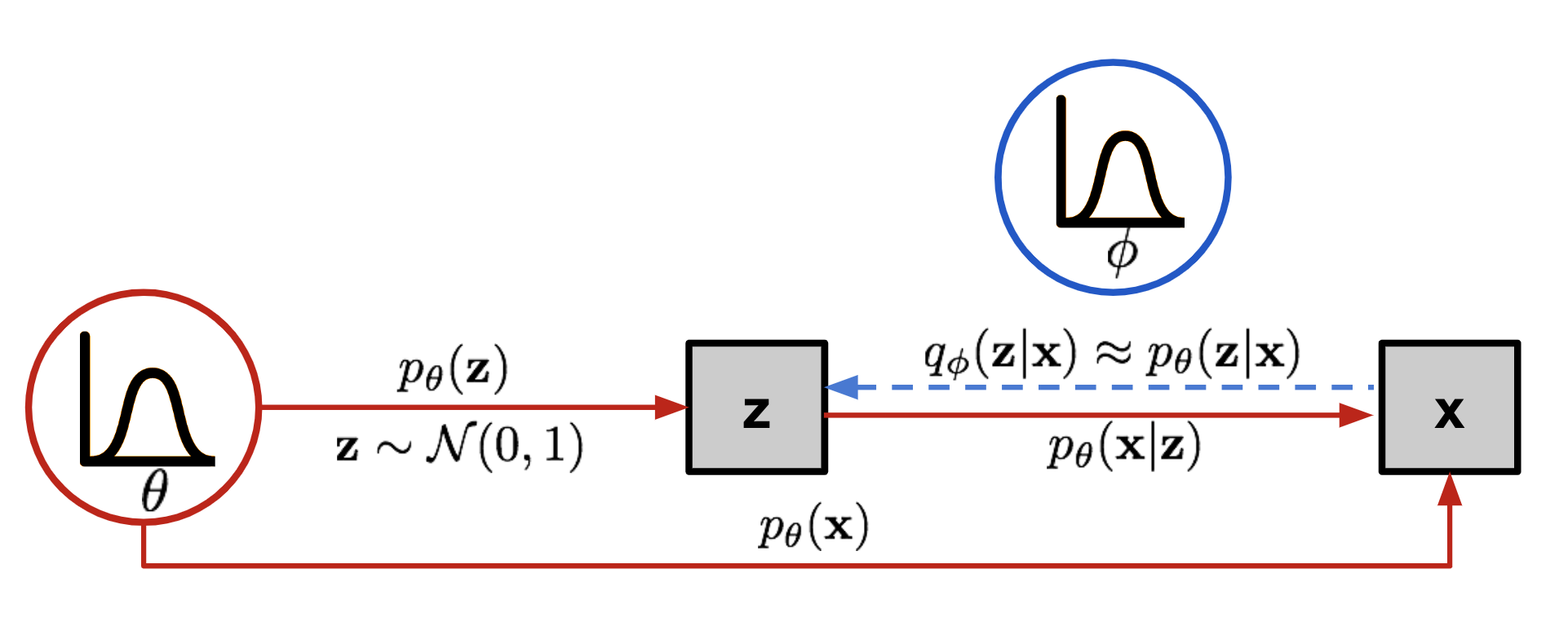
Instead of mapping the input into a fixed vector, we want to map it into a distribution. Let’s label this distribution as \(p_\theta\), parameterized by \(\theta\). The relationship between the data input \(\mathbf{x}\) and the latent encoding vector \(\mathbf{z}\) can be fully defined by:

• Prior \(p_\theta(\mathbf{z})\)
• Likelihood \(p_\theta(\mathbf{x}\vert\mathbf{z})\)
• Posterior \(p_\theta(\mathbf{z}\vert\mathbf{x})\)

如果知道分布参数 \(\theta^{*}\)，我们可以通过对 \(p_{\theta^*}(\mathbf{z})\) 采样得到 \(\mathbf{z}\)，再通过分布 \(p_{\theta^*}(\mathbf{x} \vert \mathbf{z})\) 得到一个接近真实数据的 \(\mathbf{x}\)

Assuming that we know the real parameter \(\theta^{*}\) for this distribution. In order to generate a sample that looks like a real data point \(\mathbf{x}^{(i)}\), we follow these steps:

1. First, sample a \(\mathbf{z}^{(i)}\) from a prior distribution \(p_{\theta^*}(\mathbf{z})\).
2. Then a value \(\mathbf{x}^{(i)}\) is generated from a conditional distribution \(p_{\theta^*}(\mathbf{x} \vert \mathbf{z} = \mathbf{z}^{(i)})\).

于是在给定样本集 \(\mathcal{D}\) 后，对于每个样本 \(\mathbf{x}^{(i)}\) 对应生成概率 \(p_\theta(\mathbf{x}^{(i)}) = \int p_\theta(\mathbf{x}^{(i)}\vert\mathbf{z}) p_\theta(\mathbf{z}) d\mathbf{z}\)，而这个 \(\theta^{*}\) 应当是最大似然的：

The optimal parameter \(\theta^{*}\) is the one that maximizes the probability of generating real data samples:

\[\begin{aligned} \theta^{*} &= \arg\max_\theta \prod_{i=1}^n p_\theta(\mathbf{x}^{(i)}) \\ &= \arg\max_\theta \sum_{i=1}^n \log p_\theta(\mathbf{x}^{(i)}) \\ \end{aligned} \]

where

\[p_\theta(\mathbf{x}^{(i)}) = \int p_\theta(\mathbf{x}^{(i)}\vert\mathbf{z}) p_\theta(\mathbf{z}) {\rm d}\mathbf{z} \]

不过这种计算方法并不好算，我们引入一个新的分布 \(q_\phi(\mathbf{z}\vert\mathbf{x})\)，用来拟合 \(p_\theta(\mathbf{z}\vert\mathbf{x})\)

Unfortunately it is not easy to compute \(p_\theta(\mathbf{x}^{(i)})\) in this way, as it is very expensive to check all the possible values of \(\mathbf{z}\) and sum them up. To narrow down the value space to facilitate faster search, we would like to introduce a new approximation function to output what is a likely code given an input \(\mathbf{x}\), \(q_\phi(\mathbf{z}\vert\mathbf{x})\), parameterized by \(\phi\).

Now the structure looks a lot like an autoencoder:

• The conditional probability \(p_\theta(\mathbf{x} \vert \mathbf{z})\) defines a generative model, similar to the decoder \(f_\theta(\mathbf{x} \vert \mathbf{z})\) introduced above. \(p_\theta(\mathbf{x} \vert \mathbf{z})\) is also known as probabilistic decoder.
• The approximation function \(q_\phi(\mathbf{z} \vert \mathbf{x})\) is the probabilistic encoder, playing a similar role as \(g_\phi(\mathbf{z} \vert \mathbf{x})\) above.

Loss Function: ELBO, Evidence Lower Bound

引入一个新的分布 \(q_\phi(\mathbf{z}\vert\mathbf{x})\) 来拟合 \(p_\theta(\mathbf{z}\vert\mathbf{x})\)，我们用 KL 散度来衡量两者的相似程度，可以推导得到下面的等式

We can use Kullback-Leibler divergence to quantify the distance between these two distributions, \(q_\phi(\mathbf{z}\vert\mathbf{x})\) and \(p_\theta(\mathbf{z}\vert\mathbf{x})\). Recall that KL divergence \(D_\text{KL}(X|Y)\) measures how much information is lost if the distribution Y is used to represent X.
In our case we want to minimize \(D_\text{KL}( q_\phi(\mathbf{z}\vert\mathbf{x}) | p_\theta(\mathbf{z}\vert\mathbf{x}) )\) with respect to \(\phi\).

Why use \(D_\text{KL}(q_\phi | p_\theta)\) (reversed KL) instead of \(D_\text{KL}(p_\theta | q_\phi)\) (forward KL):
首先注意到，以 $$D_\text{KL}\Big(p(x)\Big\Vert q(x)\Big) = \int p(x)\ln \frac{p(x)}{q(x)} {\rm d}x=\mathbb{E}_{x\sim p(x)}\left[\ln \frac{p(x)}{q(x)}\right]$$ 为例，若 \(q(x)\) 在某个区域为零，而 \(p(x)\) 不为零，那么会出现 KL 散度无穷大的问题，换句话说，此时 \(q(x)\) 的非零区域是包含 \(p(x)\) 的
Forward KL divergence: \(D_\text{KL}(P|Q) = \mathbb{E}_{z\sim P(z)} \log\frac{P(z)}{Q(z)}\); we have to ensure that Q(z)>0 wherever P(z)>0. The optimized variational distribution \(q(z)\) has to cover over the entire \(p(z)\).
Reversed KL divergence: \(D_\text{KL}(Q|P) = \mathbb{E}_{z\sim Q(z)} \log\frac{Q(z)}{P(z)}\); minimizing the reversed KL divergence squeezes the \(Q(z)\) under \(P(z)\).

Let’s now expand the equation, so we have:

\[D_\text{KL}( q_\phi(\mathbf{z}\vert\mathbf{x}) \| p_\theta(\mathbf{z}\vert\mathbf{x}) ) =\log p_\theta(\mathbf{x}) + D_\text{KL}(q_\phi(\mathbf{z}\vert\mathbf{x}) \| p_\theta(\mathbf{z})) - \mathbb{E}_{\mathbf{z}\sim q_\phi(\mathbf{z}\vert\mathbf{x})}\log p_\theta(\mathbf{x}\vert\mathbf{z}) \]

Once rearrange the left and right hand side of the equation,

\[\log p_\theta(\mathbf{x}) - D_\text{KL}( q_\phi(\mathbf{z}\vert\mathbf{x}) \| p_\theta(\mathbf{z}\vert\mathbf{x}) ) = \mathbb{E}_{\mathbf{z}\sim q_\phi(\mathbf{z}\vert\mathbf{x})}\log p_\theta(\mathbf{x}\vert\mathbf{z}) - D_\text{KL}(q_\phi(\mathbf{z}\vert\mathbf{x}) \| p_\theta(\mathbf{z})) \]

等号左边第一项，就是似然取 log；第二项就是 KL 散度取负，我们自然希望等号两边越大越好；取负后，就可以作为代价函数 loss 使用

The LHS of the equation is exactly what we want to maximize when learning the true distributions: we want to maximize the (log-)likelihood of generating real data (that is \(\log p_\theta(\mathbf{x})\)) and also minimize the difference between the real and estimated posterior distributions (the term \(D_\text{KL}\) works like a regularizer). Note that \(p_\theta(\mathbf{x})\) is fixed with respect to \(q_\phi\).

So, the negation of the above defines our loss function:

\[\begin{aligned} L_\text{VAE}(\theta, \phi) &= -\log p_\theta(\mathbf{x}) + D_\text{KL}( q_\phi(\mathbf{z}\vert\mathbf{x}) \| p_\theta(\mathbf{z}\vert\mathbf{x}) )\\ &= - \mathbb{E}_{\mathbf{z} \sim q_\phi(\mathbf{z}\vert\mathbf{x})} \log p_\theta(\mathbf{x}\vert\mathbf{z}) + D_\text{KL}( q_\phi(\mathbf{z}\vert\mathbf{x}) \| p_\theta(\mathbf{z}) ) \\ \theta^{*}, \phi^{*} &= \arg\min_{\theta, \phi} L_\text{VAE} \end{aligned} \]

这里还有一个含义，当我们不断减小 loss 时，意味着似然的下界在增大

In Variational Bayesian methods, this loss function is known as the variational lower bound, or evidence lower bound. The “lower bound” part in the name comes from the fact that KL divergence is always non-negative and thus \(-L_\text{VAE}\) is the lower bound of \(\log p_\theta (\mathbf{x})\).

\[-L_\text{VAE} = \log p_\theta(\mathbf{x}) - D_\text{KL}( q_\phi(\mathbf{z}\vert\mathbf{x}) \| p_\theta(\mathbf{z}\vert\mathbf{x}) ) \leq \log p_\theta(\mathbf{x}) \]

Therefore by minimizing the loss, we are maximizing the lower bound of the probability of generating real data samples.

Reparameterization Trick

回到代价函数：

\[L_\text{VAE}(\theta, \phi) = - \mathbb{E}_{\mathbf{z} \sim q_\phi(\mathbf{z}\vert\mathbf{x})} \log p_\theta(\mathbf{x}\vert\mathbf{z}) + D_\text{KL}( q_\phi(\mathbf{z}\vert\mathbf{x}) \| p_\theta(\mathbf{z}) ) \]

分别考察两部分，前一部分求的是在 \(\mathbf{z} \sim q_\phi(\mathbf{z}\vert\mathbf{x})\) 采样下的期望，但是采样是没法求导的，所以我们改写这个分布：\(\mathbf{z} = \mathcal{T}_\phi(\mathbf{x}, \boldsymbol{\epsilon})\)，将随机的任务丢给 \(\boldsymbol{\epsilon}\)

The expectation term in the loss function invokes generating samples from \(\mathbf{z} \sim q_\phi(\mathbf{z}\vert\mathbf{x})\). Sampling is a stochastic process and therefore we cannot backpropagate the gradient. To make it trainable, the reparameterization trick is introduced: It is often possible to express the random variable \(\mathbf{z}\) as a deterministic variable \(\mathbf{z} = \mathcal{T}_\phi(\mathbf{x}, \boldsymbol{\epsilon})\), where \(\boldsymbol{\epsilon}\) is an auxiliary (辅助的) independent random variable, and the transformation function \(\mathcal{T}_\phi\) parameterized by \(\phi\) converts \(\boldsymbol{\epsilon}\) to \(\mathbf{z}\) (将 \(\boldsymbol{\epsilon}\) 转化成 \(\mathbf{z}\)).

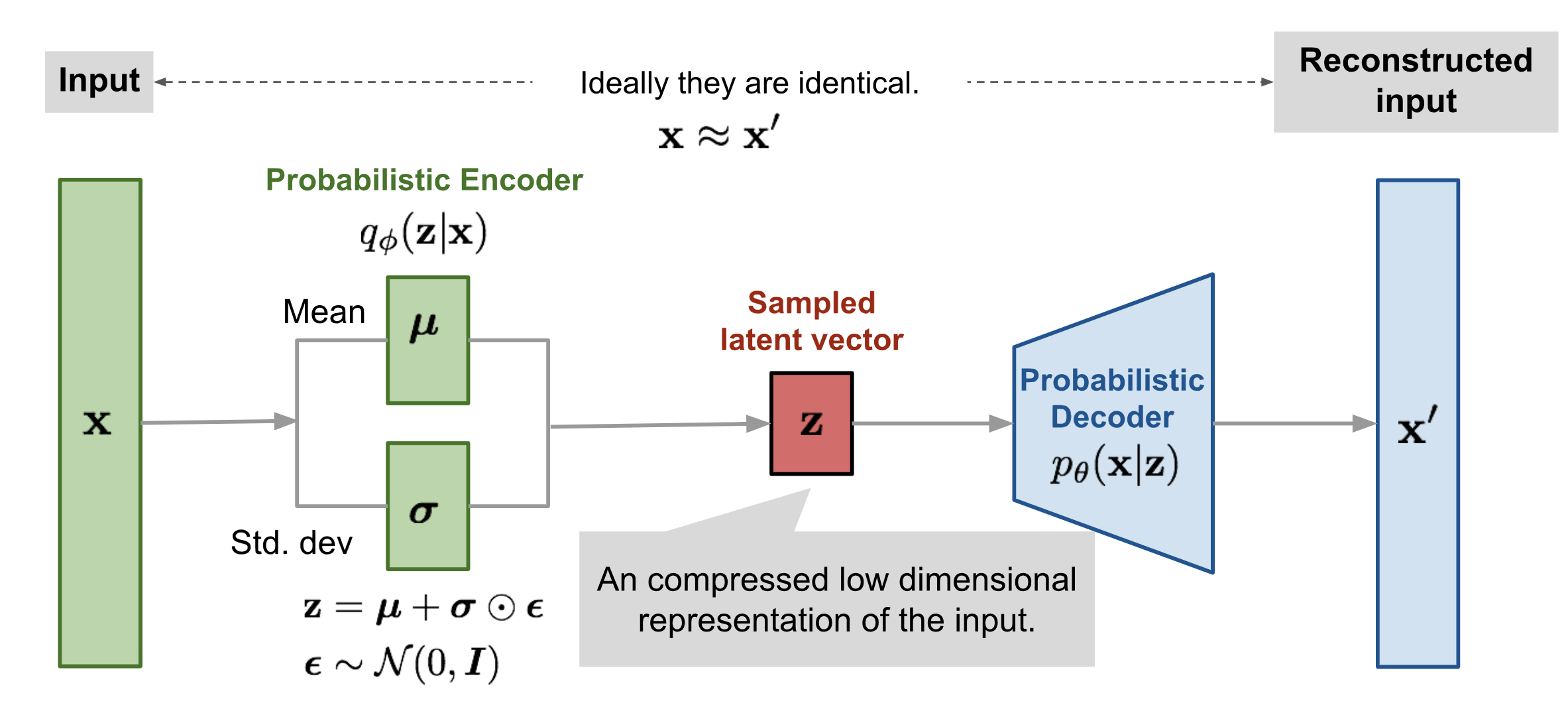
我们继续给 \(\mathcal{T}_\phi\) 一个确切形式，一般地我们选择用 多元高斯分布，而且为了方便我们假定这个高斯分布的协方差矩阵是对角阵，于是有 \(\mathbf{z} = \mathcal{T}_\phi(\mathbf{x}, \boldsymbol{\epsilon}) = \boldsymbol{\mu} + \boldsymbol{\sigma} \odot \boldsymbol{\epsilon}\)，其中 \(\boldsymbol{\mu}, \boldsymbol{\sigma}\) 是编码器学到的关于 \(\mathbf{x}\) 的输出

For example, a common choice of the form of \(q_\phi(\mathbf{z}\vert\mathbf{x})\) is a multivariate Gaussian with a diagonal covariance structure:

\[\begin{aligned} \mathbf{z} &\sim q_\phi(\mathbf{z}\vert\mathbf{x}^{(i)}) = \mathcal{N}(\mathbf{z}; \boldsymbol{\mu}^{(i)}, \boldsymbol{\sigma}^{2(i)}\boldsymbol{I}) & \\ \mathbf{z} &= \boldsymbol{\mu} + \boldsymbol{\sigma} \odot \boldsymbol{\epsilon} \text{, where } \boldsymbol{\epsilon} \sim \mathcal{N}(0, \boldsymbol{I}) & \scriptstyle{\text{; Reparameterization trick.}} \end{aligned} \]

where \(\odot\) refers to element-wise product

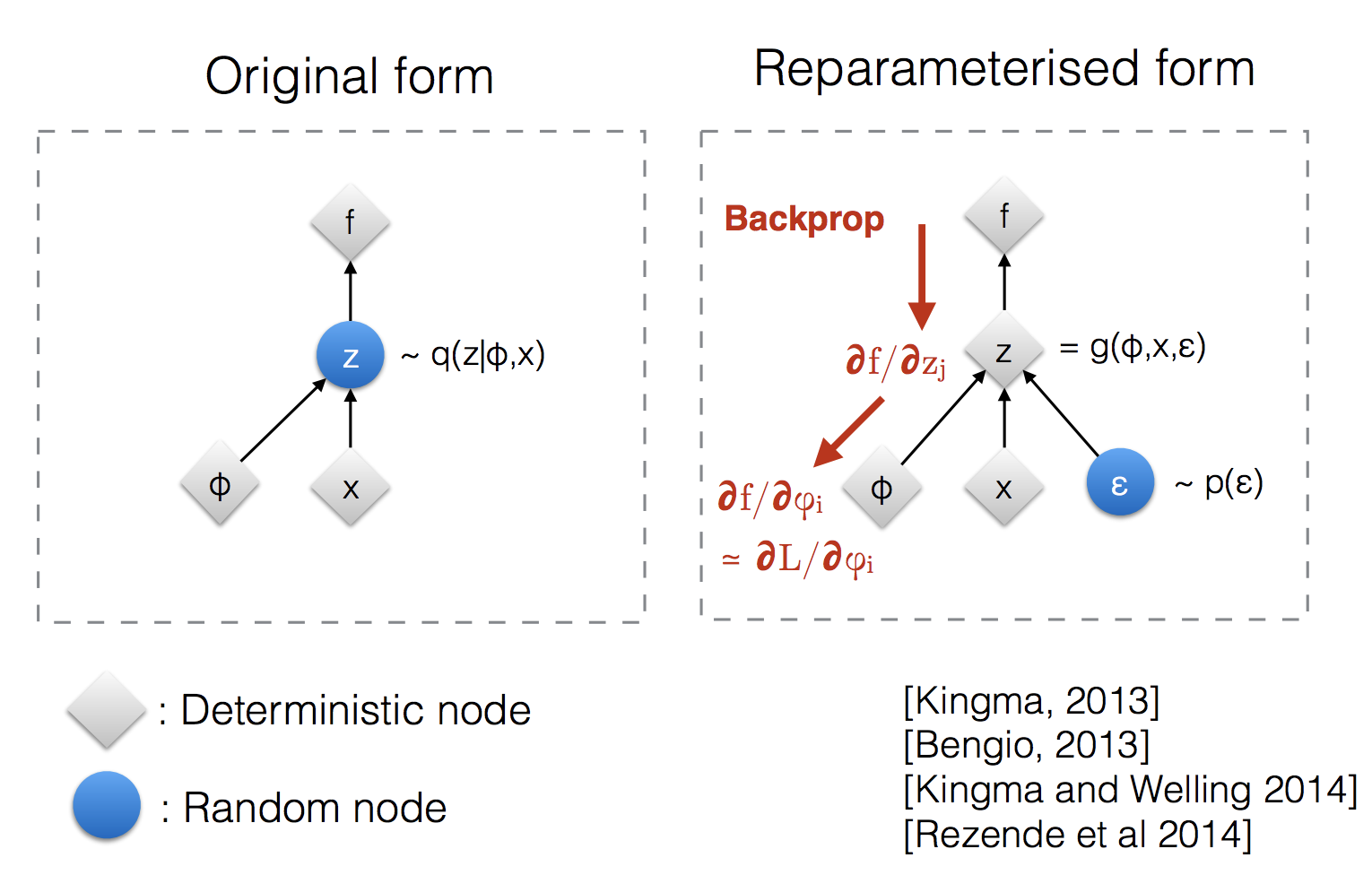
The reparameterization trick works for other types of distributions too, not only Gaussian. In the multivariate Gaussian case, we make the model trainable by learning the mean and variance of the distribution, \(\mu\) and \(\sigma\), explicitly using the reparameterization trick, while the stochasticity (随机性) remains in the random variable \(\boldsymbol{\epsilon} \sim \mathcal{N}(0, \boldsymbol{I})\).

代价函数前半部分

于是，代价函数的第一项也就成了：

\[-\mathbb{E}_{\boldsymbol{\epsilon} \sim \mathcal{N}(0, \boldsymbol{I})} \log p_\theta(\mathbf{x}\vert\mathbf{z} = \boldsymbol{\mu} + \boldsymbol{\sigma} \odot \boldsymbol{\epsilon}) \]

可是这又咋算？我们可以 采样计算，又即蒙特卡洛模拟的基础：

\[\mathbb{E}_{x\sim p(x)}[f(x)] = \int f(x)p(x)dx \approx \frac{1}{n}\sum_{i=1}^n f(x_i),\quad x_i\sim p(x) \]

那么应该采样几个呢？VAE 给出的答案是：一个！
那么代价函数的第一项就成了：

\[- \log p_\theta(\mathbf{x}\vert\mathbf{z} = \boldsymbol{\mu} + \boldsymbol{\sigma} \odot \boldsymbol{\epsilon}), \quad \boldsymbol{\epsilon} \sim \mathcal{N}(0, \boldsymbol{I}) \]

为啥只要一次呢，事实上我们会运行多个 epoch，每次的隐变量都是随机生成的，因此当 epoch 数足够多时，事实上是可以保证采样的充分性的

代价函数后半部分

此外，我们还有代价函数的后半部分呢：\(D_\text{KL}( q_\phi(\mathbf{z}\vert\mathbf{x}) \| p_\theta(\mathbf{z}) )\)

其中 \(\mathbf{z} \sim q_\phi(\mathbf{z}\vert\mathbf{x}^{(i)}) = \mathcal{N}(\mathbf{z}; \boldsymbol{\mu}^{(i)}, \boldsymbol{\sigma}^{2(i)}\boldsymbol{I})\) 是我们已经做好的，后者呢？我们直接认为，\(\mathbf{z}\) 服从标准正态分布，如此简单的假设也是注意到 “任何 d 维分布都可以从一个 d 维高斯分布 + 一个足够复杂的函数映射得到”，足够复杂的函数就当作交给解码器了
还有另一种理解，VAE 期望所有 \(q_\phi(\mathbf{z}\vert\mathbf{x})\)，或者说 \(p_\theta(\mathbf{z}\vert\mathbf{x})\) 趋近于标准正态分布，那么就会有 \(\mathbf{z}\) 趋近正态分布，这样就能保证我们之后能通过在标准正态分布中采样 \(\mathbf{z}\) 来做生成了，所以令 \(p_\theta(\mathbf{z})\) 为标准正态做的 KL 散度，也是为了让 \(q_\phi(\mathbf{z}\vert\mathbf{x})\) 趋近正态分布的正则项

那么我们在做的就是求两个高斯分布的 KL 散度，有公式：

\[\begin{aligned} &D_\text{KL}(\mathcal{N}(\boldsymbol{\mu_0}, \boldsymbol{\Sigma_0}) \| \mathcal{N}(\boldsymbol{\mu_1}, \boldsymbol{\Sigma_1})) \\ =& \frac{1}{2}\bigg( \text{tr}(\boldsymbol{\Sigma_1}^{-1} \boldsymbol{\Sigma_0}) + (\boldsymbol{\mu_1}-\boldsymbol{\mu_0})^T\boldsymbol{\Sigma_1}^{-1}(\boldsymbol{\mu_1}-\boldsymbol{\mu_0}) - d + \log\frac{\det \boldsymbol{\Sigma_1}}{\det \boldsymbol{\Sigma_0}} \bigg) \\ =& \frac{1}{2}\bigg( \text{tr}(\boldsymbol{\sigma}^{2(i)}\boldsymbol{I}) + \boldsymbol{\mu}^{(i)T}\boldsymbol{\mu}^{(i)} - d - \log \det (\boldsymbol{\sigma}^{2(i)}\boldsymbol{I}) \bigg) & \text{; $\boldsymbol{\mu_0}=\boldsymbol{\mu}^{(i)}, \boldsymbol{\Sigma_0} = \boldsymbol{\sigma}^{2(i)}\boldsymbol{I}, \boldsymbol{\mu_1}=0, \boldsymbol{\Sigma_1} = \boldsymbol{I}$} \\ \end{aligned} \]

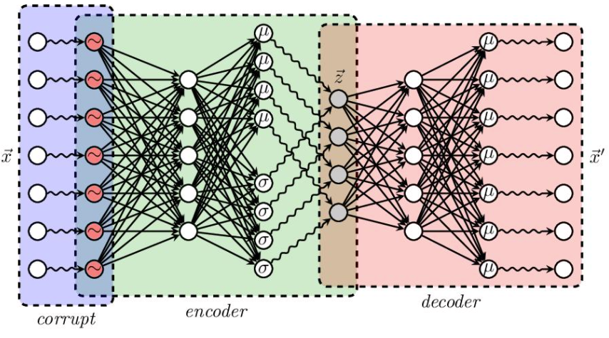
以上，我们就完成力，我们最后的神经网络长下面这样🥰
回顾，训练时我们把 \(\mathbf{x}^{(i)}\) 丢进编码器，训练输出 \(\boldsymbol{\mu}^{(i)}, \boldsymbol{\sigma}^{2(i)}\)，由 \(\mathbf{z} = \boldsymbol{\mu} + \boldsymbol{\sigma} \odot \boldsymbol{\epsilon}\) 采样一次 \(\boldsymbol{\epsilon}\) 得到 \(\mathbf{z}\)
再把 \(\mathbf{z}\) 丢进解码器，即 \(p_\theta(\mathbf{x} \vert \mathbf{z})\)，得到 \(\mathbf{x}'^{(i)}\)

代价函数的另一种理解

在看到 这个理解 前，我以为代价函数的式子纯粹就是上面的等式移项得到的，但是这个式子可以从另一个角度感性理解，重新观察代价函数：

\[L_\text{VAE}(\theta, \phi) = - \mathbb{E}_{\mathbf{z} \sim q_\phi(\mathbf{z}\vert\mathbf{x})} \log p_\theta(\mathbf{x}\vert\mathbf{z}) + D_\text{KL}( q_\phi(\mathbf{z}\vert\mathbf{x}) \| \mathcal{N}(0,\boldsymbol{I}) ) \]

前者（带负号）是解码器 \(p_\theta(\mathbf{x}\vert\mathbf{z})\) 的重构误差，也就是解码器重构出的 \(\mathbf{x}'\) 和扔进去的 \(\mathbf{x}\) 的差异，是为了提高拟合程度的；后者是编码器 \(q_\phi(\mathbf{z}\vert\mathbf{x})\) 和期望的正态分布的差异，其中均值部分担任了编码任务，方差部分调节了噪声强度，从而使得具有一定的生成能力
重构和噪声两者是对立的，最终的结果就会是，\(p_\theta(\mathbf{x}\vert\mathbf{z})\) 保留了一定的 \(\mathbf{x}\) 信息，重构效果也还可以，并且标准正态分布的假设近似成立，所以同时保留着生成能力。

Conditional VAE - 条件 VAE

考虑把标签数据加进去辅助生成样本，得到的一类模型

一种实现方法是，在前面的讨论中，我们希望 \(\mathbf{x}\) 经过编码后，\(\mathbf{z}\) 的分布都具有零均值和单位方差，这个“希望”是通过加入了 KL loss 来实现的。如果现在多了类别信息 \(\mathbf{Y}\)，我们可以希望同一个类的样本都有一个专属的均值 \(\mathbf{μ}^\mathbf{Y}\)（方差不变，还是单位方差），这个 \(\mathbf{μ}^\mathbf{Y}\) 让模型自己训练出来。这样的话，有多少个类就有多少个正态分布，而在生成的时候，我们就可以通过控制均值来控制生成图像的类别。事实上，这个“新希望”也只需通过修改 KL loss 实现：

\[\mathcal{L}_{\mathbf{\mu},\mathbf{\sigma}^2}=\frac{1}{2} \sum_{i=1}^d\Big[\big(\mathbf{\mu}_{(i)}-\mathbf{\mu}^\mathbf{Y}_{(i)}\big)^2 + \mathbf{\sigma}_{(i)}^2 - \log \mathbf{\sigma}_{(i)}^2 - 1\Big] \]

实验

\(q_\phi(\mathbf{z}\vert\mathbf{x})\) 作为编码器，输入 \(\mathbf{x}\) 得到 \(\boldsymbol{\mu}, \boldsymbol{\sigma}\)
\(p_\theta(\mathbf{x}\vert\mathbf{z})\) 作为解码器，输入 \(\mathbf{z}\) 得到 \(\mathbf{x}\)

代价函数：

\[-\mathbb{E}_{\boldsymbol{\epsilon} \sim \mathcal{N}(0, \boldsymbol{I})} \log p_\theta(\mathbf{x}\vert\mathbf{z} = \boldsymbol{\mu} + \boldsymbol{\sigma} \odot \boldsymbol{\epsilon}) + \frac{1}{2}\bigg( \text{tr}(\boldsymbol{\sigma}^{2(i)}\boldsymbol{I}) + \boldsymbol{\mu}^{(i)T}\boldsymbol{\mu}^{(i)} - d - \log \det (\boldsymbol{\sigma}^{2(i)}\boldsymbol{I}) \bigg) \]

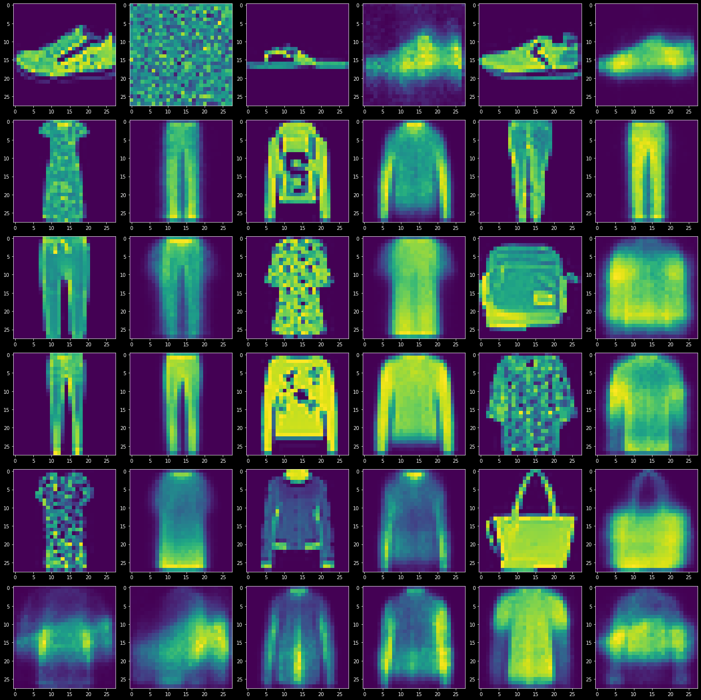
用 FashionMNIST 数据集，看看会得到什么🤗🤗🤗

import torch
from torch import nn
from torchvision import datasets
from torch.utils.data import DataLoader
from torchvision.transforms import ToTensor
import torch.nn.functional as F

import matplotlib.pyplot as plt

BATCH_SIZE = 64
original_dim = 28 * 28
intermediate_dim = 256
latent_dim = 16

train_data = datasets.FashionMNIST(root="../../data", train=True, download=False, transform=ToTensor())
train_dataloader = DataLoader(train_data, batch_size=BATCH_SIZE, shuffle=True)

class VAE(nn.Module):
    def __init__(self):
        super(VAE, self).__init__()
        self.flatten = nn.Flatten()
        self.encoder = nn.Sequential(
            nn.Linear(original_dim, intermediate_dim),
            nn.ReLU()
        )
        self.fc1 = nn.Linear(intermediate_dim, latent_dim)
        self.fc2 = nn.Linear(intermediate_dim, latent_dim)
        self.decoder = nn.Sequential(
            nn.Linear(latent_dim, intermediate_dim),
            nn.ReLU(),
            nn.Linear(intermediate_dim, original_dim),
            nn.Sigmoid()
        )
    def sampling(self, mu, logvar):
        return mu + torch.exp(logvar/2) * torch.randn(mu.shape)
    def forward(self, x):
        x = self.flatten(x)
        param = self.encoder(x)
        mu, logvar = self.fc1(param), self.fc2(param)
        z = self.sampling(mu, logvar)
        return x, self.decoder(z), mu, logvar

def loss_fn(x, est_x, mu, logvar): # notice the order in cross_entropy !
    loss1 = F.binary_cross_entropy(est_x, x, size_average=False) # By default the losses are averaged over each loss element in the batch.
    loss2 = 0.5 * torch.sum(logvar.exp() + mu.pow(2) - 1 - logvar)
    return loss1 + loss2

model_vae = VAE()
optimizer =  torch.optim.Adam(model_vae.parameters(), lr=1e-4, betas=(0.9, 0.999), eps=1e-8, weight_decay=0)

def train_loop(epoch, dataloader, model, loss_fn, optimizer):
    size = len(dataloader.dataset)
    for batch, (x, _) in enumerate(dataloader):
        x, est_x, mu, logvar = model(x)
        loss = loss_fn(x, est_x, mu, logvar)
        
        optimizer.zero_grad()
        loss.backward()
        optimizer.step()
        
        if batch % 400 == 0:
            loss, current = loss.item(), batch * len(x)
            print(f"loss: {loss:>7f}  [{current:>5d}/{size:>5d}]")
            img = x[0].data.view(28, 28)
            est_img = est_x[0].data.view(28, 28)
            axes[epoch, batch//300*2].imshow(img)
            axes[epoch, batch//300*2+1].imshow(est_img)

EPOCH, FRAME = 5, 6
fig, axes = plt.subplots(EPOCH + 1, FRAME)

for epoch in range(EPOCH):
    print(f"\nEpoch {epoch+1}\n-------------------------------")
    train_loop(epoch, train_dataloader, model_vae, loss_fn, optimizer)
print("\nfinished!")

for index in range(FRAME):
    z = torch.randn(latent_dim)
    est_x = model_vae.decoder(z)
    est_img = est_x.data.view(28, 28)
    axes[EPOCH, index].imshow(est_img)

fig.set_size_inches(20, 20)
fig.tight_layout()
plt.show()

运行结果：

Epoch 1
-------------------------------
loss: 35166.300781  [    0/60000]
loss: 19889.992188  [25600/60000]
loss: 18840.707031  [51200/60000]

Epoch 2
-------------------------------
loss: 18221.738281  [    0/60000]
loss: 17805.244141  [25600/60000]
...
loss: 16657.718750  [    0/60000]
loss: 16280.100586  [25600/60000]
loss: 16884.894531  [51200/60000]

finished!

如下，前5行，逐行边训练边输出一组原图+生成图，最后一行是直接从标准正态取样再生成
虽然像素本来就不高，但是真的好糊...😰😰😰