
《机器学习Python实现_09_01_决策树_ID3与C4.5》
简介
先看一个例子,某银行是否给用户放贷的判断规则集如下:
if 年龄==青年:
    if 有工作==是:
        if 信贷情况==非常好:
            放
        else:
            不放
    else:
        if 有自己的房子==是:
            if 信贷情况==一般:
                不放
            else:
                放
        else:
            if 信贷情况==非常好 or 信贷情况==好:
                放
            else:
                if 有工作==是:
                    放
                else:
                    不放
elif 年龄==中年:
    if 有自己的房子==是:
        放
    else:
        if 信贷情况==非常好 or 信贷情况==好:
            放
        else:
            if 有工作==是:
                放
            else:
                不放
elif 年龄==老年:
    if 有自己的房子==是:
        if 信贷情况==非常好 or 信贷情况==好:
            放
        else:
            不放
    else:
        if 信贷情况==非常好 or 信贷情况==好:
            if 有工作==是:
                放
            else:
                不放
        else:
            不放
if 有自己的房子==是:
    放
else:
    if 有工作==是:
        放
    else:
        不放
眼力好的同学立马会发现这代码写的有问题,比如只要信贷情况==非常好的用户都有放款,何必嵌到里面去?而且很多规则有冗余,为什么不重构一下呀?但现实情况是你可能真不敢随意乱动!因为指不定哪天项目经理又要新增加规则了,所以宁可让代码越来越冗余,越来越复杂,也不敢随意乱动之前的规则,乱动两条,可能会带来意想不到的灾难。简单总结一下这种复杂嵌套的if else规则可能存在的痛点:
(1)规则可能不完备,存在某些匹配不上的情况;
(2)规则之间存在冗余,多个if else情况其实是判断的同样的条件;
(3)严重时,可能会出现矛盾的情况,即相同的条件,即有放,又有不放;
(4)判断规则的优先级混乱,比如信贷情况因子可以优先考虑,因为只要它是非常好就可以放款,而不必先判断其它条件
而决策树算法就能解决以上痛点,它能保证所有的规则互斥且完备,即用户的任意一种情况一定能匹配上一条规则,且该规则唯一,这样就能解决上面的痛点1~3,且规则判断的优先级也很不错,下面介绍决策树学习算法。
决策树学习
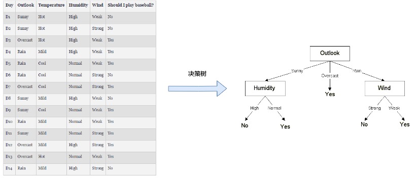
决策树算法可以从已标记的数据中自动学习出if else规则集,如下图(图片来源>>>),左边是收集的一系列判断是否打球的案例,包括4个特征outlook,temperature,Humidity,Wind,以及y标签是否打球,通过决策树学习后得到右边的决策树,决策树的结构如图所示,它由节点和有向边组成,而节点又分为两种:叶子节点和非叶子节点,非叶子节点主要用于对某一特征做判断,而它下面所链接的有向边表示该特征所满足的某条件,最终的叶子节点即表示实例的预测值(分类/回归)
决策树学习主要分为两个阶段,决策树生成和决策树剪枝,决策树生成阶段最重要便是特征选择,下面对相关概念做介绍:
1.特征选择
特征选择用于选择对分类有用的特征,ID3和C4.5通常选择的准则是信息增益和信息增益比,下面对其作介绍并实现
信息增益
首先介绍两个随机变量之间的互信息公式:
这里\(H(X)\)表示\(X\)的熵,在最大熵模型那一节已做过介绍:
条件熵\(H(Y|X)\)表示在已知随机变量\(X\)的条件下,随机变量\(Y\)的不确定性:
而信息增益就是\(Y\)取分类标签,\(X\)取某一特征时的互信息,它表示如果选择特征\(X\)对数据进行分割,可以使得分割后\(Y\)分布的熵降低多少,若降低的越多,说明分割每个子集的\(Y\)的分布越集中,则\(X\)对分类标签\(Y\)越有用,下面进行python实现:
"""
定义计算熵的函数,封装到ml_models.utils
"""
import numpy as np
from collections import Counter
import math
def entropy(x,sample_weight=None):
    x=np.asarray(x)
    #x中元素个数
    x_num=len(x)
    #如果sample_weight为None设均设置一样
    if sample_weight is None:
        sample_weight=np.asarray([1.0]*x_num)
    x_counter={}
    weight_counter={}
    # 统计各x取值出现的次数以及其对应的sample_weight列表
    for index in range(0,x_num):
        x_value=x[index]
        if x_counter.get(x_value) is None:
            x_counter[x_value]=0
            weight_counter[x_value]=[]
        x_counter[x_value]+=1
        weight_counter[x_value].append(sample_weight[index])

    #计算熵
    ent=.0
    for key,value in x_counter.items():
        p_i=1.0*value*np.mean(weight_counter.get(key))/x_num
        ent+=-p_i*math.log(p_i)
    return ent
#测试
entropy([1,2])
0.6931471805599453
def cond_entropy(x, y,sample_weight=None):
    """
    计算条件熵:H(y|x)
    """
    x=np.asarray(x)
    y=np.asarray(y)
    # x中元素个数
    x_num = len(x)
    #如果sample_weight为None设均设置一样
    if sample_weight is None:
        sample_weight=np.asarray([1.0]*x_num)
    # 计算
    ent = .0
    for x_value in set(x):
        x_index=np.where(x==x_value)
        new_x=x[x_index]
        new_y=y[x_index]
        new_sample_weight=sample_weight[x_index]
        p_i=1.0*len(new_x)/x_num
        ent += p_i * entropy(new_y,new_sample_weight)
    return ent
#测试
cond_entropy([1,2],[1,2])
0.0
def muti_info(x, y,sample_weight=None):
    """
    互信息/信息增益:H(y)-H(y|x)
    """
    x_num=len(x)
    if sample_weight is None:
        sample_weight=np.asarray([1.0]*x_num)
    return entropy(y,sample_weight) - cond_entropy(x, y,sample_weight)
接下来,做一个测试,看特征的取值的个数对信息增益的影响
import random
import numpy as np
import matplotlib.pyplot as plt
%matplotlib inline
#作epochs次测试
epochs=100
#x的取值的个数:2->class_num_x
class_num_x=100
#y标签类别数
class_num_y=2
#样本数量
num_samples=500
info_gains=[]
for _ in range(0,epochs):
    info_gain=[]
    for class_x in range(2,class_num_x):
        x=[]
        y=[]
        for _ in range(0,num_samples):
            x.append(random.randint(1,class_x))
            y.append(random.randint(1,class_num_y))
        info_gain.append(muti_info(x,y))
    info_gains.append(info_gain)
plt.plot(np.asarray(info_gains).mean(axis=0))
[<matplotlib.lines.Line2D at 0x21ed2625ba8>]
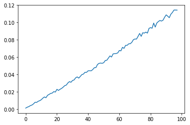
可以发现一个很有意思的现象,如果特征的取值的个数越多,越容易被选中,这比较好理解,假设一个极端情况,若对每一个实例特征\(x\)的取值都不同,则其\(H(Y|X)\)项为0,则\(MI(X,Y)=H(Y)-H(Y|X)\)将会取得最大值(\(H(Y)\)与\(X\)无关),这便是ID3算法的一个痛点,为了矫正这一问题,C4.5算法利用信息增益比作特征选择
信息增益比
信息增益比其实就是对信息增益除以了一个\(x\)的熵:
def info_gain_rate(x, y,sample_weight=None):
    """
    信息增益比
    """
    x_num=len(x)
    if sample_weight is None:
        sample_weight=np.asarray([1.0]*x_num)
    return 1.0 * muti_info(x, y,sample_weight) / (1e-12 + entropy(x,sample_weight))
接下来再作一次相同的测试:
#作epochs次测试
epochs=100
#x的取值的个数:2->class_num_x
class_num_x=100
#y标签类别数
class_num_y=2
#样本数量
num_samples=500
info_gain_rates=[]
for _ in range(0,epochs):
    info_gain_rate_=[]
    for class_x in range(2,class_num_x):
        x=[]
        y=[]
        for _ in range(0,num_samples):
            x.append(random.randint(1,class_x))
            y.append(random.randint(1,class_num_y))
        info_gain_rate_.append(info_gain_rate(x,y))
    info_gain_rates.append(info_gain_rate_)
plt.plot(np.asarray(info_gain_rates).mean(axis=0))
[<matplotlib.lines.Line2D at 0x21ed26da978>]
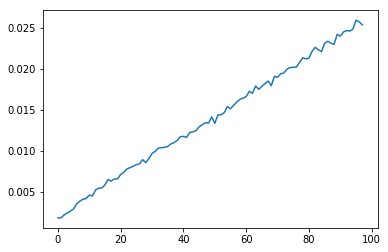
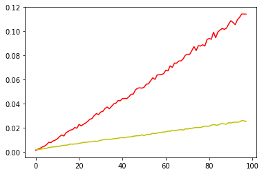
虽然整体还是上升的趋势,当相比于信息增益已经缓解了很多,将它们画一起直观感受一下:
plt.plot(np.asarray(info_gains).mean(axis=0),'r')
plt.plot(np.asarray(info_gain_rates).mean(axis=0),'y')
[<matplotlib.lines.Line2D at 0x21ed267e860>]
2.决策树生成
决策树的生成就是一个递归地调用特征选择的过程,首先从根节点开始,利用信息增益/信息增益比选择最佳的特征作为节点特征,由该特征的不同取值建立子节点,然后再对子节点调用以上方法,直到所有特征的信息增益/信息增益比均很小或者没有特征可以选择时停止,最后得到一颗决策树。接下来直接进行代码实现:
import os
os.chdir('../')
from ml_models import utils
from ml_models.wrapper_models import DataBinWrapper
"""
ID3和C4.5决策树分类器的实现,放到ml_models.tree模块
"""
class DecisionTreeClassifier(object):
    class Node(object):
        """
        树节点,用于存储节点信息以及关联子节点
        """

        def __init__(self, feature_index: int = None, target_distribute: dict = None, weight_distribute: dict = None,
                     children_nodes: dict = None, num_sample: int = None):
            """
            :param feature_index: 特征id
            :param target_distribute: 目标分布
            :param weight_distribute:权重分布
            :param children_nodes: 孩子节点
            :param num_sample:样本量
            """
            self.feature_index = feature_index
            self.target_distribute = target_distribute
            self.weight_distribute = weight_distribute
            self.children_nodes = children_nodes
            self.num_sample = num_sample

    def __init__(self, criterion='c4.5', max_depth=None, min_samples_split=2, min_samples_leaf=1,
                 min_impurity_decrease=0, max_bins=10):
        """
        :param criterion:划分标准,包括id3,c4.5,默认为c4.5
        :param max_depth:树的最大深度
        :param min_samples_split:当对一个内部结点划分时,要求该结点上的最小样本数,默认为2
        :param min_samples_leaf:设置叶子结点上的最小样本数,默认为1
        :param min_impurity_decrease:打算划分一个内部结点时,只有当划分后不纯度(可以用criterion参数指定的度量来描述)减少值不小于该参数指定的值,才会对该结点进行划分,默认值为0
        """
        self.criterion = criterion
        if criterion == 'c4.5':
            self.criterion_func = utils.info_gain_rate
        else:
            self.criterion_func = utils.muti_info
        self.max_depth = max_depth
        self.min_samples_split = min_samples_split
        self.min_samples_leaf = min_samples_leaf
        self.min_impurity_decrease = min_impurity_decrease

        self.root_node: self.Node = None
        self.sample_weight = None
        self.dbw = DataBinWrapper(max_bins=max_bins)

    def _build_tree(self, current_depth, current_node: Node, x, y, sample_weight):
        """
        递归进行特征选择,构建树
        :param x:
        :param y:
        :param sample_weight:
        :return:
        """
        rows, cols = x.shape
        # 计算y分布以及其权重分布
        target_distribute = {}
        weight_distribute = {}
        for index, tmp_value in enumerate(y):
            if tmp_value not in target_distribute:
                target_distribute[tmp_value] = 0.0
                weight_distribute[tmp_value] = []
            target_distribute[tmp_value] += 1.0
            weight_distribute[tmp_value].append(sample_weight[index])
        for key, value in target_distribute.items():
            target_distribute[key] = value / rows
            weight_distribute[key] = np.mean(weight_distribute[key])
        current_node.target_distribute = target_distribute
        current_node.weight_distribute = weight_distribute
        current_node.num_sample = rows
        # 判断停止切分的条件

        if len(target_distribute) <= 1:
            return

        if rows < self.min_samples_split:
            return

        if self.max_depth is not None and current_depth > self.max_depth:
            return

        # 寻找最佳的特征
        best_index = None
        best_criterion_value = 0
        for index in range(0, cols):
            criterion_value = self.criterion_func(x[:, index], y)
            if criterion_value > best_criterion_value:
                best_criterion_value = criterion_value
                best_index = index

        # 如果criterion_value减少不够则停止
        if best_index is None:
            return
        if best_criterion_value <= self.min_impurity_decrease:
            return
        # 切分
        current_node.feature_index = best_index
        children_nodes = {}
        current_node.children_nodes = children_nodes
        selected_x = x[:, best_index]
        for item in set(selected_x):
            selected_index = np.where(selected_x == item)
            # 如果切分后的点太少,以至于都不能做叶子节点,则停止分割
            if len(selected_index[0]) < self.min_samples_leaf:
                continue
            child_node = self.Node()
            children_nodes[item] = child_node
            self._build_tree(current_depth + 1, child_node, x[selected_index], y[selected_index],
                             sample_weight[selected_index])

    def fit(self, x, y, sample_weight=None):
        # check sample_weight
        n_sample = x.shape[0]
        if sample_weight is None:
            self.sample_weight = np.asarray([1.0] * n_sample)
        else:
            self.sample_weight = sample_weight
        # check sample_weight
        if len(self.sample_weight) != n_sample:
            raise Exception('sample_weight size error:', len(self.sample_weight))

        # 构建空的根节点
        self.root_node = self.Node()

        # 对x分箱
        self.dbw.fit(x)

        # 递归构建树
        self._build_tree(1, self.root_node, self.dbw.transform(x), y, self.sample_weight)

    # 检索叶子节点的结果
    def _search_node(self, current_node: Node, x, class_num):
        if current_node.feature_index is None or current_node.children_nodes is None or len(
                current_node.children_nodes) == 0 or current_node.children_nodes.get(
            x[current_node.feature_index]) is None:
            result = []
            total_value = 0.0
            for index in range(0, class_num):
                value = current_node.target_distribute.get(index, 0) * current_node.weight_distribute.get(index, 1.0)
                result.append(value)
                total_value += value
            # 归一化
            for index in range(0, class_num):
                result[index] = result[index] / total_value
            return result
        else:
            return self._search_node(current_node.children_nodes.get(x[current_node.feature_index]), x, class_num)

    def predict_proba(self, x):
        # 计算结果概率分布
        x = self.dbw.transform(x)
        rows = x.shape[0]
        results = []
        class_num = len(self.root_node.target_distribute)
        for row in range(0, rows):
            results.append(self._search_node(self.root_node, x[row], class_num))
        return np.asarray(results)

    def predict(self, x):
        return np.argmax(self.predict_proba(x), axis=1)
#造伪数据
from sklearn.datasets import make_classification
data, target = make_classification(n_samples=100, n_features=2, n_classes=2, n_informative=1, n_redundant=0,
                                   n_repeated=0, n_clusters_per_class=1, class_sep=.5,random_state=21)
#训练查看效果
tree = DecisionTreeClassifier(max_bins=15)
tree.fit(data, target)
utils.plot_decision_function(data, target, tree)
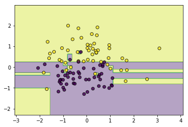
可以发现,如果不对决策树施加一些限制,它会尝试创造很细碎的规则去使所有的训练样本正确分类,这无疑会使得模型过拟合,所以接下来需要对其进行减枝操作,避免其过拟合
3.决策树剪枝
顾名思义,剪掉一些不必要的叶子节点,那么如何确定那些叶子节点需要去掉,哪些不需要去掉呢?这可以通过构建损失函数来量化,如果剪掉某一叶子结点后损失函数能减少,则进行剪枝操作,如果不能减少则不剪枝。一种简单的量化损失函数可以定义如下:
这里\(\mid T \mid\)表示树\(T\)的叶结点个数,\(t\)是树\(\mid T \mid\)的叶结点,该叶节点有\(N_t\)个样本点,其中\(k\)类样本点有\(N_{tk}\)个,\(k=1,2,3,...,K\),\(H_t(T)\)为叶结点\(t\)上的经验熵,\(\alpha\geq 0\)为超参数,其中:
该损失函数可以分为两部分,第一部分\(\sum_{t=1}^{\mid T\mid}N_tH_t(T)\)为经验损失,第二部分\(\mid T \mid\)为结构损失,\(\alpha\)为调节其平衡度的系数,如果\(\alpha\)越大则模型结构越简单,越不容易过拟合,接下来进行剪枝的代码实现:
    def _prune_node(self, current_node: Node, alpha):
        # 如果有子结点,先对子结点部分剪枝
        if current_node.children_nodes is not None and len(current_node.children_nodes) != 0:
            for child_node in current_node.children_nodes.values():
                self._prune_node(child_node, alpha)

        # 再尝试对当前结点剪枝
        if current_node.children_nodes is not None and len(current_node.children_nodes) != 0:
            # 避免跳层剪枝
            for child_node in current_node.children_nodes.values():
                # 当前剪枝的层必须是叶子结点的层
                if child_node.children_nodes is not None and len(child_node.children_nodes) > 0:
                    return
            # 计算剪枝前的损失值
            pre_prune_value = alpha * len(current_node.children_nodes)
            for child_node in current_node.children_nodes.values():
                for key, value in child_node.target_distribute.items():
                    pre_prune_value += -1 * child_node.num_sample * value * np.log(
                        value) * child_node.weight_distribute.get(key, 1.0)
            # 计算剪枝后的损失值
            after_prune_value = alpha
            for key, value in current_node.target_distribute.items():
                after_prune_value += -1 * current_node.num_sample * value * np.log(
                    value) * current_node.weight_distribute.get(key, 1.0)

            if after_prune_value <= pre_prune_value:
                # 剪枝操作
                current_node.children_nodes = None
                current_node.feature_index = None

    def prune(self, alpha=0.01):
        """
        决策树剪枝 C(T)+alpha*|T|
        :param alpha:
        :return:
        """
        # 递归剪枝
        self._prune_node(self.root_node, alpha)
from ml_models.tree import DecisionTreeClassifier
#训练查看效果
tree = DecisionTreeClassifier(max_bins=15)
tree.fit(data, target)
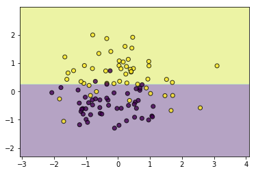
tree.prune(alpha=1.5)
utils.plot_decision_function(data, target, tree)

通过探索\(\alpha\),我们可以得到一个比较令人满意的剪枝结果,这样的剪枝方式通常又被称为后剪枝,即从一颗完整生成后的树开始剪枝,与其对应的还有预剪枝,即在训练过程中就对其进行剪枝操作,这通常需要另外构建一份验证集做支持,这里就不实现了,另外比较通常的做法是,通过一些参数来控制模型的复杂度,比如max_depth控制树的最大深度,min_samples_leaf控制叶子结点的最小样本数,min_impurity_decrease控制特征划分后的最小不纯度,min_samples_split控制结点划分的最小样本数,通过调节这些参数,同样可以达到剪枝的效果,比如下面通过控制叶结点的最小数量达到了和上面剪枝一样的效果:
tree = DecisionTreeClassifier(max_bins=15,min_samples_leaf=3)
tree.fit(data, target)
utils.plot_decision_function(data, target, tree)
决策树另外一种理解:条件概率分布
决策树还可以看作是给定特征条件下类的条件概率分布:
(1)训练时,决策树会将特征空间划分为大大小小互不相交的区域,而每个区域对应了一个类的概率分布;
(2)预测时,落到某区域的样本点的类标签即是该区域对应概率最大的那个类
作者: 努力的番茄
出处: https://www.cnblogs.com/zhulei227/
关于作者:专注于机器学习、深度学习、强化学习、NLP等领域!
本文版权归作者和博客园共有,欢迎转载,但未经作者同意必须保留此段声明,且在文章页面明显位置给出.

 浙公网安备 33010602011771号