数据分析之描述性统计

1 导入数据

import pandas as pd 
import numpy as np 
import matplotlib.pyplot as plt 
import seaborn as sns

iris = sns.load_dataset('iris')

<class 'pandas.core.frame.DataFrame'>
RangeIndex: 150 entries, 0 to 149
Data columns (total 5 columns):
 #   Column        Non-Null Count  Dtype  
---  ------        --------------  -----  
 0   sepal_length  150 non-null    float64
 1   sepal_width   150 non-null    float64
 2   petal_length  150 non-null    float64
 3   petal_width   150 non-null    float64
 4   species       150 non-null    object 
dtypes: float64(4), object(1)
memory usage: 6.0+ KB

2 查新数据概况

2.1 查看总体统计信息

# 查看数据基本信息
iris.info()

# 查看前几行
iris.head()

# 查看后几行
iris.tail()

# 查看连续变量数据的统计特征,
iris.describe()

# 查看分类变量的统计特征
iris.species.value_counts()

<class 'pandas.core.frame.DataFrame'>
RangeIndex: 150 entries, 0 to 149
Data columns (total 5 columns):
 #   Column        Non-Null Count  Dtype  
---  ------        --------------  -----  
 0   sepal_length  150 non-null    float64
 1   sepal_width   150 non-null    float64
 2   petal_length  150 non-null    float64
 3   petal_width   150 non-null    float64
 4   species       150 non-null    object 
dtypes: float64(4), object(1)
memory usage: 6.0+ KB





setosa        50
versicolor    50
virginica     50
Name: species, dtype: int64

# 计算各变量的方差（variance）
iris.var()

# 考察各变量之间的相关系数矩阵
iris.corr()

	sepal_length	sepal_width	petal_length	petal_width
sepal_length	1.000000	-0.117570	0.871754	0.817941
sepal_width	-0.117570	1.000000	-0.428440	-0.366126
petal_length	0.871754	-0.428440	1.000000	0.962865
petal_width	0.817941	-0.366126	0.962865	1.000000

结果显示，花萼宽度（sepal_width）与其他三个变量花萼长度（sepal_length）、花瓣长度（petal_length）、花瓣宽度（petal_width）均为负相关，似乎有些奇怪。但这可能是因为样本中混杂了三种不同的鸢尾花品种。为此，将iris数据框按照变量species的取值进行分组。

2.2 查看分组统计信息

iris_grouped = iris.groupby('species')

# 查看相关系数
iris_grouped.corr()

# 显示所有列
pd.set_option("display.max_columns", None)

# 查看所有分组的统计指标
iris_grouped.describe()

# 查看petal_length变量的统计指标
iris_grouped.petal_length.describe()

		sepal_length	sepal_width	petal_length	petal_width
species
setosa	sepal_length	1.000000	0.742547	0.267176	0.278098
	sepal_width	0.742547	1.000000	0.177700	0.232752
	petal_length	0.267176	0.177700	1.000000	0.331630
	petal_width	0.278098	0.232752	0.331630	1.000000
versicolor	sepal_length	1.000000	0.525911	0.754049	0.546461
	sepal_width	0.525911	1.000000	0.560522	0.663999
	petal_length	0.754049	0.560522	1.000000	0.786668
	petal_width	0.546461	0.663999	0.786668	1.000000
virginica	sepal_length	1.000000	0.457228	0.864225	0.281108
	sepal_width	0.457228	1.000000	0.401045	0.537728
	petal_length	0.864225	0.401045	1.000000	0.322108
	petal_width	0.281108	0.537728	0.322108	1.000000

结果显示，在控制了鸢尾花品种之后，所有变量之间的相关系数均为正数。对于此分组数据，使用describe()方法，可得到每个品种的统计指标。

# 查看所有变量的分组平均值
iris_grouped.mean()

# 计算所有变量的分组平均值与分组标准差，使用agg()方差（表示aggregate，即合计）
iris_grouped.agg(['mean', 'median', 'std'])

# 计算不同变量的统计值
iris_grouped.agg({'sepal_length': 'mean', 'sepal_width': 'mean', 'petal_length': 'std', 'petal_width': 'std'})

# 自定义四分位距指标
def iqr(x):
    return x.quantile(0.75) - x.quantile(0.25)
iris_grouped.agg(iqr)

	sepal_length			sepal_width			petal_length			petal_width
	mean	std	median	mean	std	median	mean	std	median	mean	std	median
species
setosa	5.006	0.352490	5.0	3.428	0.379064	3.4	1.462	0.173664	1.50	0.246	0.105386	0.2
versicolor	5.936	0.516171	5.9	2.770	0.313798	2.8	4.260	0.469911	4.35	1.326	0.197753	1.3
virginica	6.588	0.635880	6.5	2.974	0.322497	3.0	5.552	0.551895	5.55	2.026	0.274650	2.0

# 对原始数据进行分组标准化，使得每组数据的均值均为0而标准差为1
def zscore(x):
    return (x-x.mean()) / x.std()

transformed = iris_grouped.transform(zscore)
transformed.head(3)

# 对变换后的数据框transformed，考察期均值与标准差
transformed.groupby(iris.species).agg(['mean', 'std'])

	sepal_length		sepal_width		petal_length		petal_width
	mean	std	mean	std	mean	std	mean	std
species
setosa	1.872044e-15	1.0	-2.167155e-15	1.0	-1.159073e-15	1.0	9.192647e-16	1.0
versicolor	7.882583e-17	1.0	-1.513234e-15	1.0	4.640732e-16	1.0	8.204548e-16	1.0
virginica	2.766676e-15	1.0	7.413514e-16	1.0	6.283862e-16	1.0	6.639134e-16	1.0

3 直观展示

画图的库主要有：Matplotlib与seaborn，另外pandas自带的也有画图工具，下面结合使用：

3.1 使用pandas的hist()方法画直方图

# 查看sepal_length的分布情况，即查看直方图
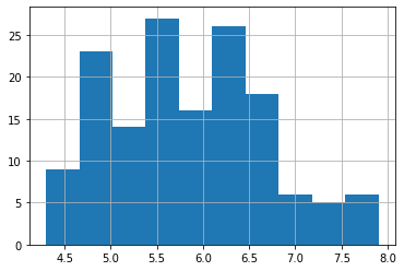
iris.sepal_length.hist()  #默认分为10组

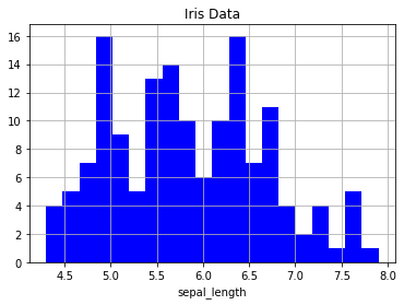
# 直方图，将数据分为20组，使用蓝色画图，并添加标签与标题
iris.sepal_length.hist(bins=20, color='b')
plt.xlabel('sepal_length')
plt.title('Iris Data')

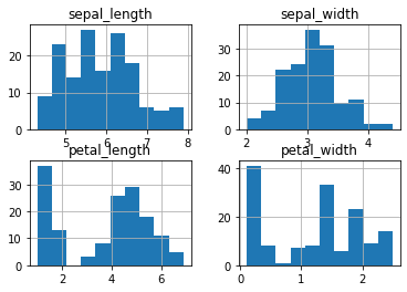
# 画所有变量的直方图
iris.hist()

3.2 核密度图

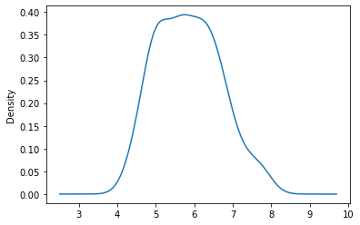
直方图估计其概率密度分布的密度函数（density function），所得结果既不光滑也不连续，因而使用核密度图进行估计。

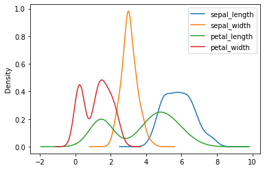
iris.sepal_length.plot.density()

# 画所有变量的和密度图
iris.plot.density()

# 每个变量画在不同的图中
iris.plot.density(subplots=True)

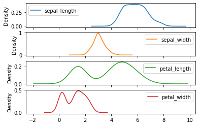
如图所示，花萼长度（sepal_length）与宽度（sepal_width）的核密度为单峰分布，而花瓣长度（petal_length）与宽度（petal_width）的核密度图则呈现双峰分布。

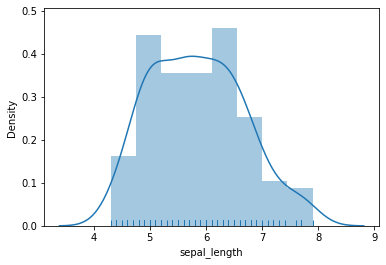
# 同时画sepal_length的直方图与核密度图
sns.distplot(iris.sepal_length, rug=True)

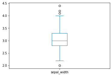
3.3 箱型图

箱型图主要用于查看数据的异常值分布

箱体的上边界为四分之三分位数（upper quartile），下边界为四分之一分位数（lower quartile），而箱体中部的横线为中位数（median）。箱体上方的横线为“上边缘”（upper hinge），其到箱体上边界（upper quartile）的距离为箱体高度的1.5倍；而箱体下方的横线为“下边缘”（lower hinger），其到箱体下边界(lower quartile）的距离也是箱体高度的1.5倍。所有上边缘与下边缘之外的观测值均可视为“极端值”或“离群值”（outliers），在图中以空心小圆点表示。箱型图可以非常简洁地概括出一个变量的分布特征。

iris.sepal_width.plot.box()

# 画所有变量的箱型图
iris.plot.box()

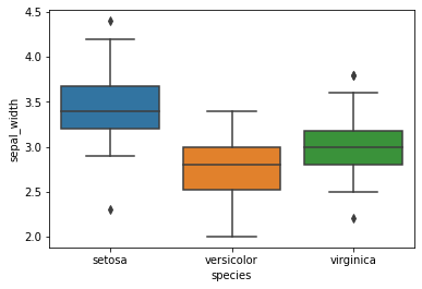
# 由于四个特征变量的取值分布与波动幅度不尽相同，因此同时画三个不同品种（species）的鸢尾花的花萼宽度（sepal_width）的箱型图，这需要使用seaborn库
sns.boxplot(x='species', y='sepal_width', data=iris)

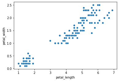
3.4 散点图

如果我们更关心变量之间的关系，而两个变量之间的散点图（scatter plot）是常用的画图工具。可用seaborn的scatterplot()函数画散点图。

sns.scatterplot(x='petal_length', y='petal_width', data=iris)

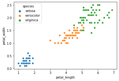
# 用不同的颜色表示不同的鸢尾花品种
sns.scatterplot(x='petal_length', y='petal_width', data=iris, hue='species')

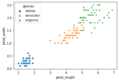
# 以不同颜色和不同图标区分鸢尾花品种
sns.scatterplot(x='petal_length', y='petal_width', data=iris, style='species', hue='species')

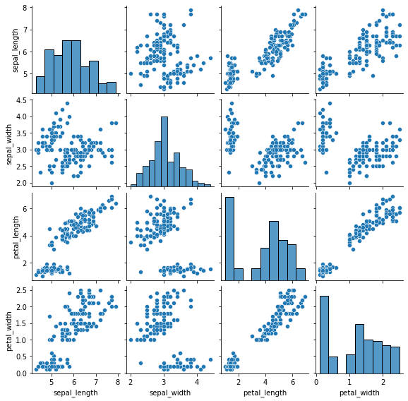
3.5 综合画图

sns.pairplot(data=iris, height=2)

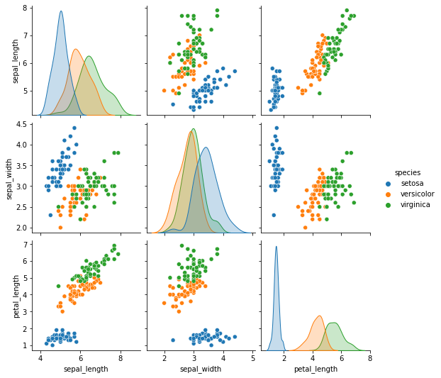
# 画部分变量的散点图，并在主对角线上画核密度图
sns.pairplot(iris, diag_kind='kde', vars=['sepal_length', 'sepal_width', 'petal_length'], hue='species')