coursera Deeplearning_1
Deeplearning在coursera总共有5章节,分别如下

1neural networks and deep learning
1.1introduction to deep learning
ReLU function: rectified linear unite 修正线性单元
1.1.1supervised learning with neural networks
some applications and their networks

最后一行autonomous driving是custom and highbrit neural network architecture
structured data: based on the database or list
1.2logistic regression as a neural network
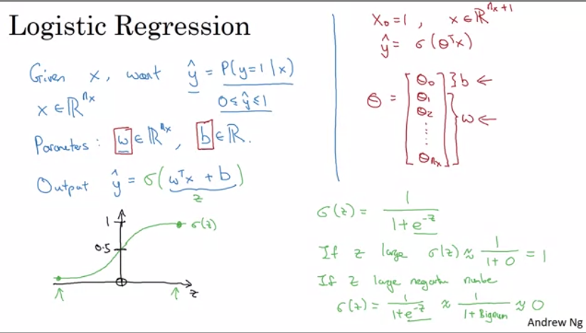
1.2.1logistic regression
在引入神经网络之前,首先搭建模型,建立logistic regression模型
output: yhat = sigma * (wT*x + b) = sigma(z) =1/(1+e^(-z))
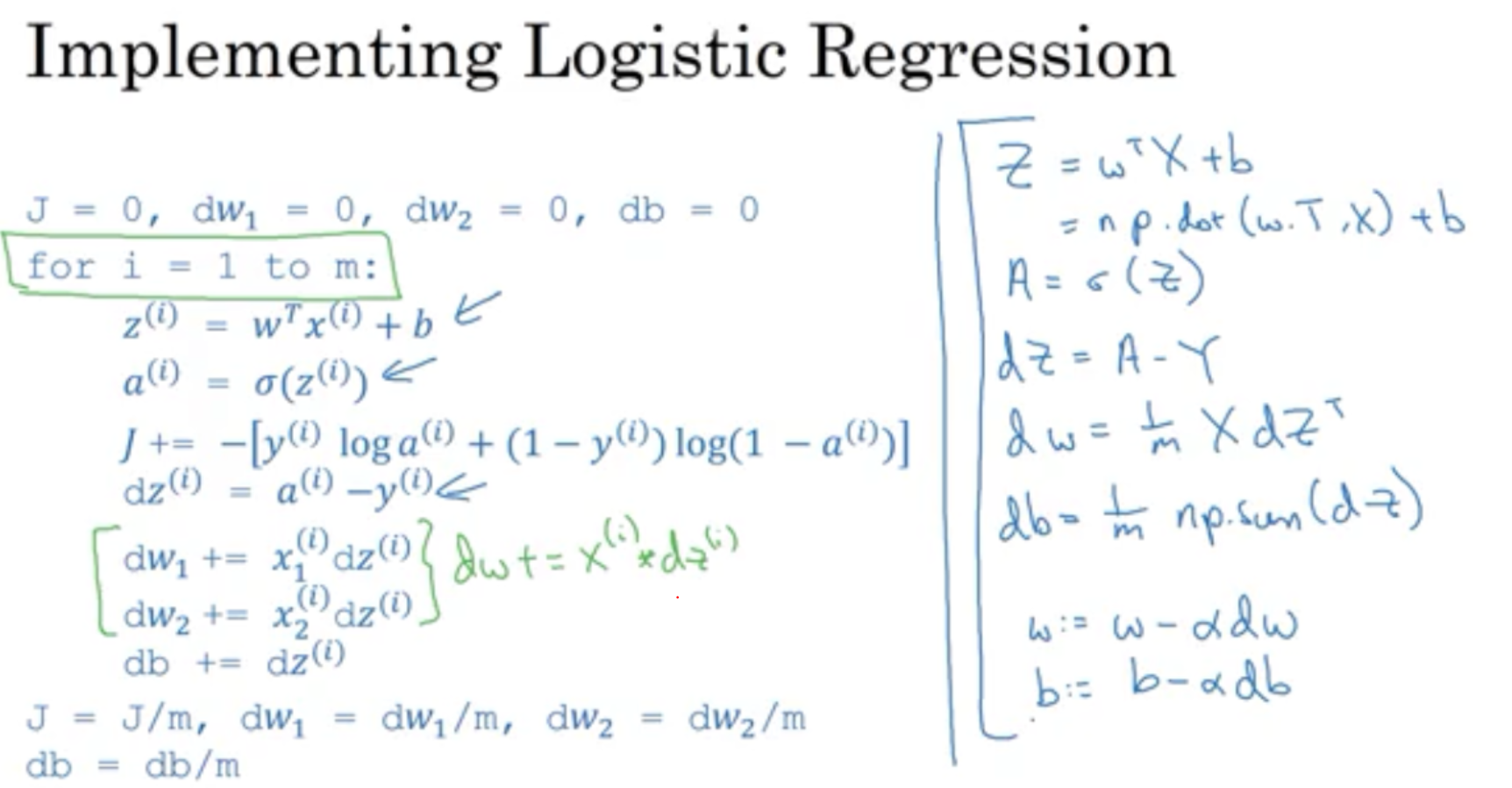
1.2.2the algorithm of Gradient descent on m examples

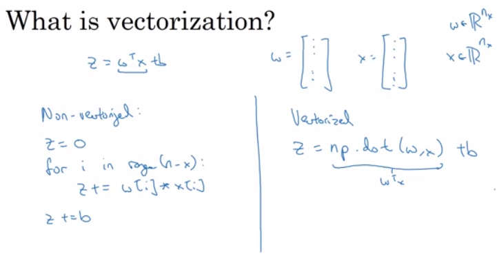
1.3python and vectorization
the difference between non-vectorization and vectorization
1.3.1jupyter代码练习之vectorization demo
- numpy求数组
import numpy as np
a = np.array([1,2,3,4])
print(a)
[1 2 3 4]
- 向量化版本


import time
a = np.random.rand(1000000)
b = np.random.rand(1000000)
tic = time.time()
c = np.dot(a,b)
toc = time.time()
print(a,b)
print("Vectorization version:"+str(1000*(toc-tic))+"ms")
[0.59467283 0.99173279 0.00123952 ... 0.29278564 0.97683776 0.8740815 ]
[0.3456192  0.29648059 0.94208957 ... 0.33763542 0.62611472 0.54614243]
Vectorization version:0.9908676147460938ms
- 向量化与循环的时间比较
import time
a = np.random.rand(1000000)
b = np.random.rand(1000000)
tic = time.time()
c = np.dot(a,b)
toc = time.time()
print(c)
print("Vectorization version:"+str(1000*(toc-tic))+"ms")

c = 0
tic = time.time()
for i in range(1000000):
    c += a[i] * b[i]
toc = time.time()
print(c)
print("For loop:"+str(1000*(toc-tic))+"ms")

249992.96116014756
Vectorization version:0.9968280792236328ms
249992.96116014617
For loop:444.3216323852539ms
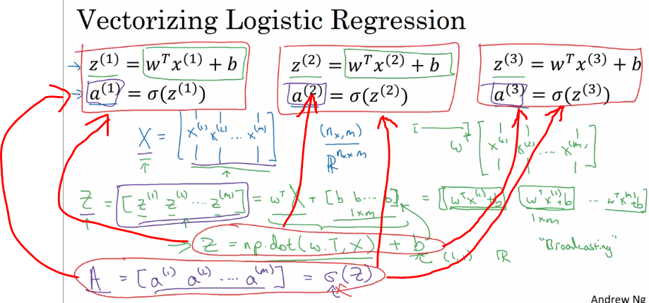
1.3.2vectoring logistic regression
对于z和a向量化后,得到z = np.dot(wT,x)+b和A=[a(1),a(2),a(3)...a(m)] = sigma(z)
1.3.3vectorizing logistic regression's gradient output
broadcasting技术
broadcasting technicals可以帮我们在运算上提高效率,有一些普通的对矩阵运算的加减乘除operation
raw vector和column vector与单一数在做np.dot运算时候区别
import numpy as np
a = np.random.randn(5)
print(a)
print(a.shape)
print(a.T)
print(np.dot(a.T,a))
a = np.random.randn(5,1)
print(a)
print(a.T)
print(np.dot(a,a.T))
[-1.25150746  0.90245975 -1.5437502  -2.03129219 -0.91442366]
(5,)
[-1.25150746  0.90245975 -1.5437502  -2.03129219 -0.91442366]
9.726187792641722
[[ 0.13143985]
 [-1.06166298]
 [-0.30208537]
 [ 0.3434191 ]
 [ 0.70496854]]
[[ 0.13143985 -1.06166298 -0.30208537  0.3434191   0.70496854]]
[[ 0.01727643 -0.13954482 -0.03970606  0.04513896  0.09266096]
 [-0.13954482  1.12712829  0.32071286 -0.36459535 -0.74843901]
 [-0.03970606  0.32071286  0.09125557 -0.10374189 -0.21296069]
 [ 0.04513896 -0.36459535 -0.10374189  0.11793668  0.24209967]
 [ 0.09266096 -0.74843901 -0.21296069  0.24209967  0.49698065]]
关于logistic regression cost function的两点推导

关于broadcasting和正常的vectorization的一些解释
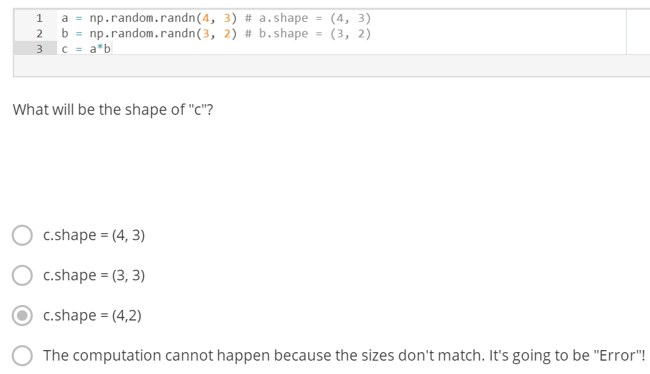
import numpy as np
a = np.random.randn(3,3)
b = np.random.randn(3,1)
print(a)
print(b)
c = a*b
d = np.dot(a,b)
print(c)
print(d)

[[ 0.7075494  -0.10429553 -0.17201322]
 [-0.53974707  0.51247682  0.42653902]
 [ 0.66015945  0.35415285  0.2497812 ]]
[[-0.01238072]
 [ 0.07473015]
 [ 0.64125908]]
[[-0.00875997  0.00129125  0.00212965]
 [-0.04033538  0.03829747  0.03187532]
 [ 0.42333324  0.22710373  0.16017446]]
[[-0.12685903]
 [ 0.31850195]
 [ 0.17846711]]
In numpy the "*" operator indicates element-wise multiplication. It is different from "np.dot()". If you would try "c = np.dot(a,b)" you would get c.shape = (4, 2).
Also, the broadcasting cannot happen because of the shape of b. b should have been something like (4, 1) or (1, 3) to broadcast properly.
element-wise multiplication 元素式乘法
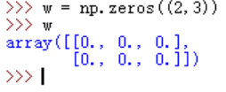
关于nump.zeros()的输出可以参考如下
2.1shadow neural network
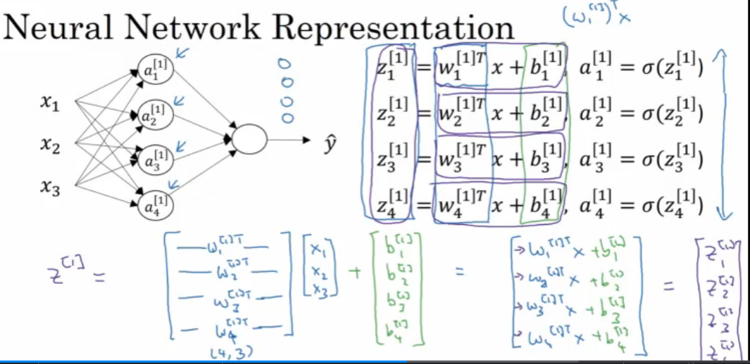
2.1.1compute a neural network's output
下图代表了第一个神经元的输出
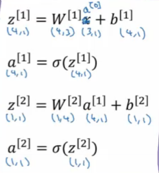
把第一个神经元的输出作为第二个神经元的输入,则可以得到如下图这样单个神经元的输出
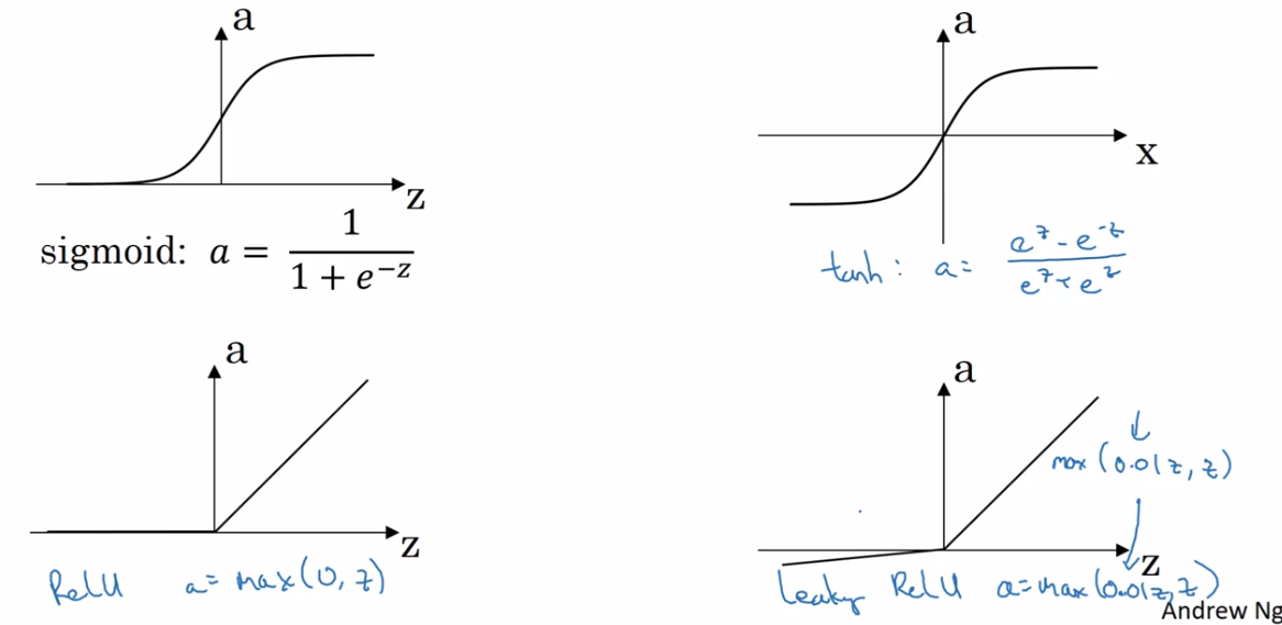
2.1.2activation function
不同activation函数
sigmoid function,tanh,ReLU(rectified linear unit), leaky ReLU
sigmoid function一般不推荐用,除非用于输出层
2.1.3non-linear activation function
因为线性隐藏层在叠加后任然是线性的,所以可以删除,而在输出的函数sigmoid function中,用非线性函数可以得到更加复杂的结果。
线性函数只会用在g(z) = z的输出层用,此时的output function可以是linear function(wb+b),但是此时需要在hidden layer中应用ReLU/tanh这种非线性函数;还有一种情况是要对数据进行压缩,会用linear function,否则很少用lin func
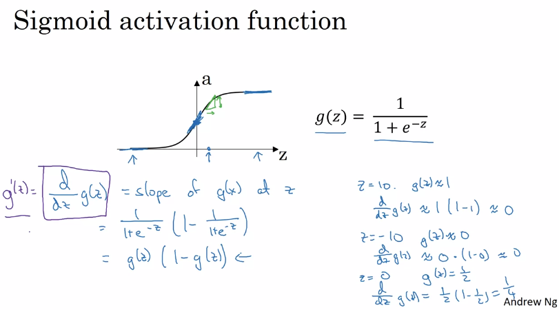
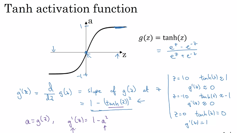
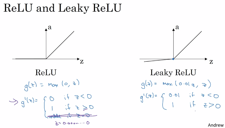
2.1.4derivatives of activation functions
sigmoid activation function
Tanh activation function
ReLU activation function
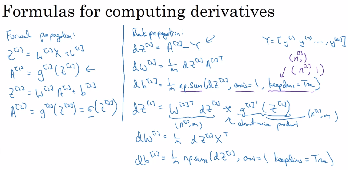
2.1.5gradient descent for neural networks
formula for computing derivatives including forward propagation and backward propagation
2.1.6back propagation intuition
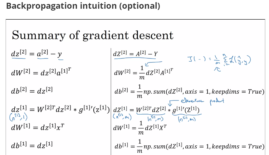
keepdims = True could ensure that the output of B is [4,1] but not [4,]
A = np.random.randn(4,3)
B = np.sum(A, axis = 1, keepdims = True)
关于输出神经元的一题
6。Suppose you have built a neural network. You decide to initialize the weights and biases to be zero.
Which of the following statements is true?
A.Each neuron in the first hidden layer will perform the same computation.
So even after multiple iterations of gradient descent each neuron in the layer will be computing the same thing as other neurons.
B.Each neuron in the first hidden layer will perform the same computation in the first iteration.
But after one iteration of gradient descent they will learn to compute different things because we have “broken symmetry”.
C.Each neuron in the first hidden layer will compute the same thing,
but neurons in different layers will compute different things, thus we have accomplished “symmetry breaking” as described in lecture.
D.The first hidden layer’s neurons will perform different computations from each other even in the first iteration;
their parameters will thus keep evolving in their own way.
解析:
如果在初始时,两个隐藏神经元的参数设置为相同的大小,那么两个隐藏神经元对输出单元的影响也是相同的,通过反向梯度下降去进行计算的时候,会
得到同样的梯度大小,所以在经过多次迭代后,两个隐藏层单位仍然是对称的。无论设置多少个隐藏单元,其最终的影响都是相同的,那么多个隐藏神经元就没有了意义。
assert函数是一个断言函数,如果条件成立,则返回true,如果条件不成立,则返回false
if(假设成立)
{
     程序正常运行;
}
else
{
      报错&&终止程序!(避免由程序运行引起更大的错误)
}
关于神经网络初始化为什么要随机,并且数值要小,可以参考这篇文章,here
关于np.power(a,b)
>>> x1 = range(6)
>>> x1
[0, 1, 2, 3, 4, 5]
>>> np.power(x1, 3)
array([  0,   1,   8,  27,  64, 125])
np.dot与np.multiply区别
np.dot()是对数组执行对应位置相乘,输出位标量,np.multiply()是依据矩阵乘法运算做运算,输出位矢量或秩为1的标量
3.1Deep L-layer neural network
神经网络设置多层,每一层多个神经元的目的:
- 对于线性不可分的数据而言,多层的神经网络的设置回归效果比softmax好;
- 对于高维数据而言,很难可视化,隐藏层的层数和每层中神经元的个数,只能通过多次调整
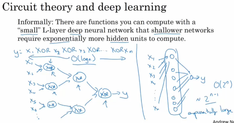
3.1.1为什么使用深层表示
如果层数多,那么算法复杂度可以达到o(log n),如果层数少,那么算法复杂度就要达到o(2^n)
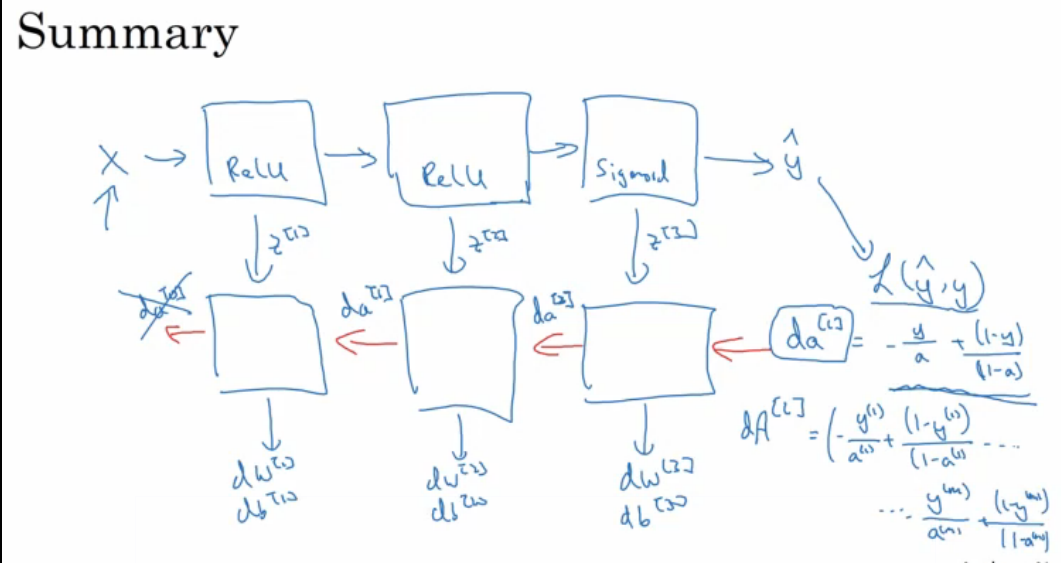
3.1.2搭建深层神经网络块
forward and backward propagation
backward propagation for layer L
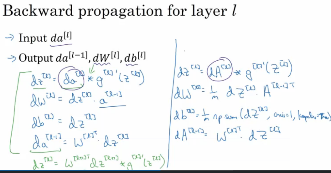
输入x,到输出loss function.
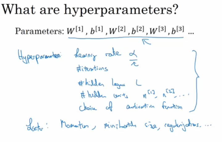
3.1.3hyperparameter
3.1.4assignment1
np.random.seed(1) is used to keep all the random function calls consistent
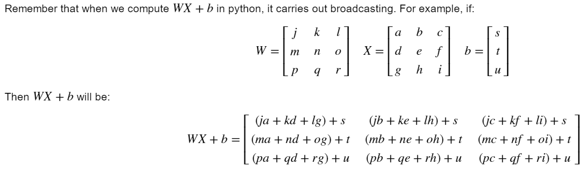
broadcasting的具体解释
3.1.5assignment2
architecture your model建立网络模型
CV识别一张图片的过程如下
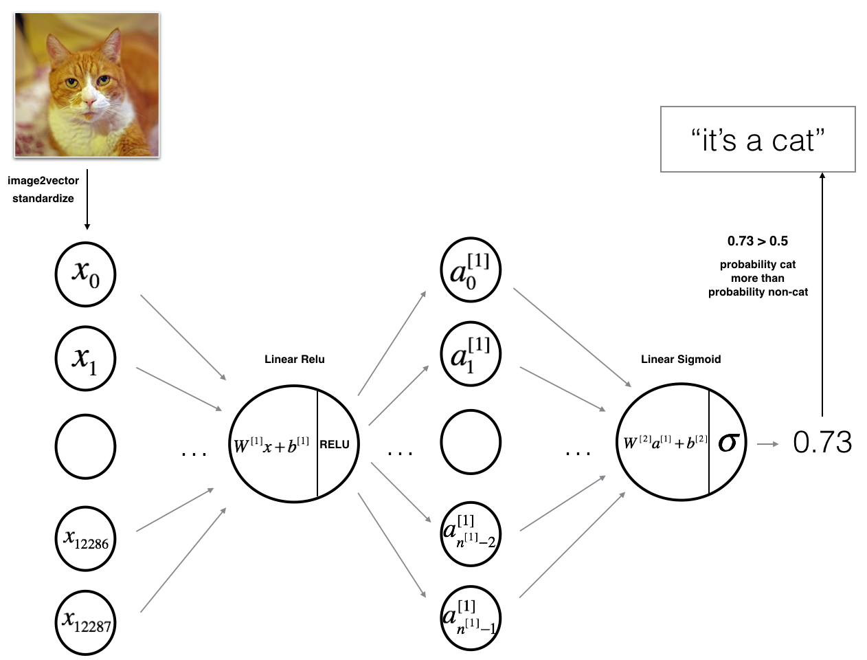
The model can be summarized as: INPUT -> LINEAR -> RELU -> LINEAR -> SIGMOID -> OUTPUT
- The input is a (64,64,3) image which is flattened to a vector of size (12288,1)(12288,1).
- The corresponding vector: [x0,x1,...,x12287]T[x0,x1,...,x12287]T is then multiplied by the weight matrix W[1]W[1] of size (n[1],12288)(n[1],12288).
- You then add a bias term and take its relu to get the following vector: [a[1]0,a[1]1,...,a[1]n[1]−1]T[a0[1],a1[1],...,an[1]−1[1]]T.
- You then repeat the same process.
- You multiply the resulting vector by W[2]W[2] and add your intercept (bias).
- Finally, you take the sigmoid of the result. If it is greater than 0.5, you classify it to be a cat.
操作后的结果
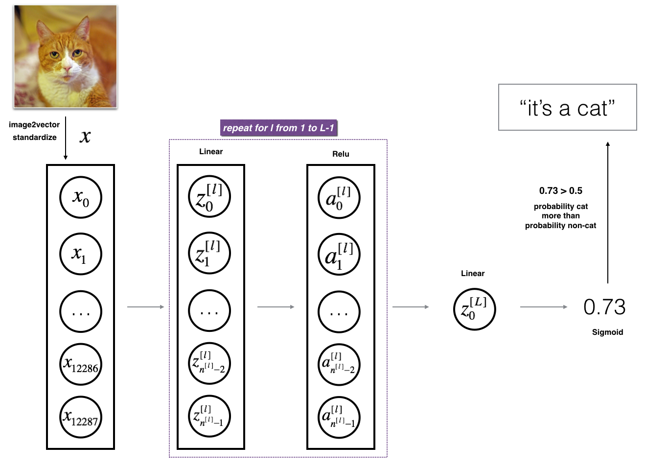
[LINEAR -> RELU] ×× (L-1) -> LINEAR -> SIGMOID
- The input is a (64,64,3) image which is flattened to a vector of size (12288,1).
- The corresponding vector: [x0,x1,...,x12287]T[x0,x1,...,x12287]T is then multiplied by the weight matrix W[1]W[1] and then you add the intercept b[1]b[1]. The result is called the linear unit.
- Next, you take the relu of the linear unit. This process could be repeated several times for each (W[l],b[l])(W[l],b[l]) depending on the model architecture.
- Finally, you take the sigmoid of the final linear unit. If it is greater than 0.5, you classify it to be a cat.、


 浙公网安备 33010602011771号