第九周作业

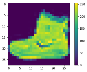
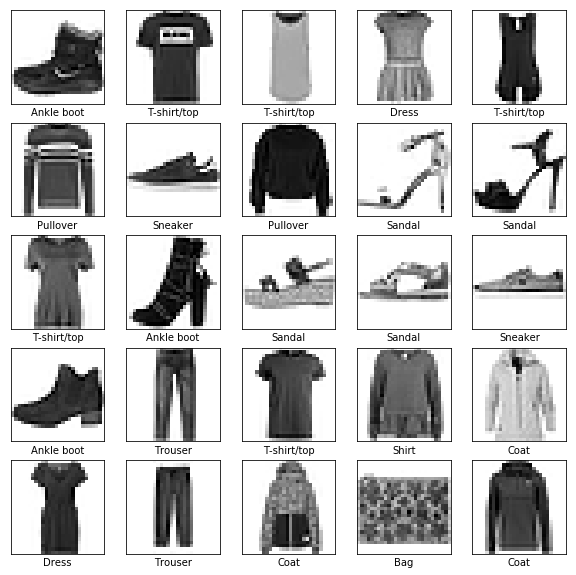
import tensorflow as tf
from tensorflow import keras

# Helper libraries
import numpy as np
import matplotlib.pyplot as plt

print(tf.__version__)
fashion_mnist = keras.datasets.fashion_mnist

(train_images, train_labels), (test_images, test_labels) = fashion_mnist.load_data()
fashion_mnist = keras.datasets.fashion_mnist

class_names = ['T-shirt/top', 'Trouser', 'Pullover', 'Dress', 'Coat',
               'Sandal', 'Shirt', 'Sneaker', 'Bag', 'Ankle boot']
len(train_labels)


len(test_labels)
plt.figure()
plt.imshow(train_images[0])
plt.colorbar()
plt.grid(False)
plt.show()
train_images = train_images / 255.0

test_images = test_images / 255.0
plt.figure(figsize=(10,10))
for i in range(25):
    plt.subplot(5,5,i+1)
    plt.xticks([])
    plt.yticks([])
    plt.grid(False)
    plt.imshow(train_images[i], cmap=plt.cm.binary)
    plt.xlabel(class_names[train_labels[i]])
plt.show()
model = keras.Sequential([
    keras.layers.Flatten(input_shape=(28, 28)),
    keras.layers.Dense(128, activation='relu'),
    keras.layers.Dense(10)
])
model.compile(optimizer='adam',
              loss=tf.keras.losses.SparseCategoricalCrossentropy(from_logits=True),
              metrics=['accuracy'])
model.fit(train_images, train_labels, epochs=10)
test_loss, test_acc = model.evaluate(test_images,  test_labels, verbose=2)

print('\nTest accuracy:', test_acc)
probability_model = tf.keras.Sequential([model,
                                         tf.keras.layers.Softmax()])
predictions = probability_model.predict(test_images)

np.argmax(predictions[0])

def plot_image(i, predictions_array, true_label, img):
  predictions_array, true_label, img = predictions_array, true_label[i], img[i]
  plt.grid(False)
  plt.xticks([])
  plt.yticks([])

  plt.imshow(img, cmap=plt.cm.binary)

  predicted_label = np.argmax(predictions_array)
  if predicted_label == true_label:
    color = 'blue'
  else:
    color = 'red'

  plt.xlabel("{} {:2.0f}% ({})".format(class_names[predicted_label],
                                100*np.max(predictions_array),
                                class_names[true_label]),
                                color=color)

def plot_value_array(i, predictions_array, true_label):
  predictions_array, true_label = predictions_array, true_label[i]
  plt.grid(False)
  plt.xticks(range(10))
  plt.yticks([])
  thisplot = plt.bar(range(10), predictions_array, color="#777777")
  plt.ylim([0, 1])
  predicted_label = np.argmax(predictions_array)

  thisplot[predicted_label].set_color('red')
  thisplot[true_label].set_color('blue')
i = 0
plt.figure(figsize=(6, 3))
plt.subplot(1, 2, 1)
plot_image(i, predictions[i], test_labels, test_images)
plt.subplot(1, 2, 2)
plot_value_array(i, predictions[i], test_labels)
plt.show()
i = 12
plt.figure(figsize=(6, 3))
plt.subplot(1, 2, 1)
plot_image(i, predictions[i], test_labels, test_images)
plt.subplot(1, 2, 2)
plot_value_array(i, predictions[i], test_labels)
plt.show()
# Plot the first X test images, their predicted labels, and the true labels.
# Color correct predictions in blue and incorrect predictions in red.
num_rows = 5
num_cols = 3
num_images = num_rows * num_cols
plt.figure(figsize=(2 * 2 * num_cols, 2 * num_rows))
for i in range(num_images):
    plt.subplot(num_rows, 2 * num_cols, 2 * i + 1)
    plot_image(i, predictions[i], test_labels, test_images)
    plt.subplot(num_rows, 2 * num_cols, 2 * i + 2)
    plot_value_array(i, predictions[i], test_labels)
plt.tight_layout()
plt.show()
# Grab an image from the test dataset.
img = test_images[1]

print(img.shape)
# Add the image to a batch where it's the only member.
img = (np.expand_dims(img, 0))

print(img.shape)
predictions_single = probability_model.predict(img)

print(predictions_single)
plot_value_array(1, predictions_single[0], test_labels)
_ = plt.xticks(range(10), class_names, rotation=45)
np.argmax(predictions_single[0])

 

 

 

6.5习题

1.局部连接：层间神经只有局部范围内的连接，在这个范围内采用全连接的方式，超过这个范围的神经元则没有连接；连接与连接之间独立参数，相比于去全连接减少了感受域外的连接，有效减少参数规模。

全连接：层间神经元完全连接，每个输出神经元可以获取到所有神经元的信息，有利于信息汇总，常置于网络末尾；连接与连接之间独立参数，大量的连接大大增加模型的参数规模。

 

2.先需要把img转成矩阵格式。

①先计算卷积输出图像的尺寸，上图中的 HxW；

②从图像的左上角处开始滑动，窗口大小为卷积核的大小(如3x3的卷积核，就从原img最左上角的那3x3区域开始，把3x3拉成一条变1x9，放入col中)，然后stride移动，得到 HxW个1x9横条，将他们往纵向(下)堆；上图中一列的红/绿/蓝

③因为输入是多维度的(caffe中是HxWxC)，那么在C channel上也要堆叠，channel 方向上则是一张张单维img往横向(右)堆；上图中每一行的红/绿/蓝，这样就得到 feature matrix：HxW x CxKxK

对卷积核 Filter 也同样做矩阵转换，得到 Cout x CxKxK (Cout为输出的channel，卷积核的个数)。img和filter都转成矩阵后，就可以进行矩阵乘法了：filter matrix * (feature matrix)T    CoutxHxW = Cout x CxKxK * (CxKxK x HxW)    (CxKxK x HxW) 为img矩阵的转置。

 

3.池化的作用：对输入的特征图进行压缩，一方面使特征图变小，简化网络计算复杂度；一方面进行特征压缩，提取主要特征。

激活函数的作用：如果不用激励函数，每一层输出都是上层输入的线性函数，无论神经网络有多少层，输出都是输入的线性组合。
如果使用的话，激活函数给神经元引入了非线性因素，使得神经网络可以任意逼近任何非线性函数，这样神经网络就可以应用到众多的非线性模型中。

 

4.①归一化有助于快速收敛②对局部神经元的活动创建竞争机制，使得其中响应比较大的值变得相对更大，并抑制其他反馈较小的神经元，增强了模型的泛化能力。

 

5.寻找损失函数的最低点