【笔记】机器学习 - 李宏毅 - 2 - Regression + Demo

Regression 回归
应用领域包括：Stock Market Forecast, Self-driving car, Recommondation,...

Step 1: Model

对于宝可梦的CP值预测问题，假设为一个最简单的线性模型
y = b + \(\sum w_i x_i\)
\(x_i\): an attribute of input x(feature)
\(w_i\): weight, b: bias

Step 2: Goodness of Function

定义一个Loss Function来评价Function的好坏，
（input: a function, output: how bad it is, L(f) = L(w, b) ）

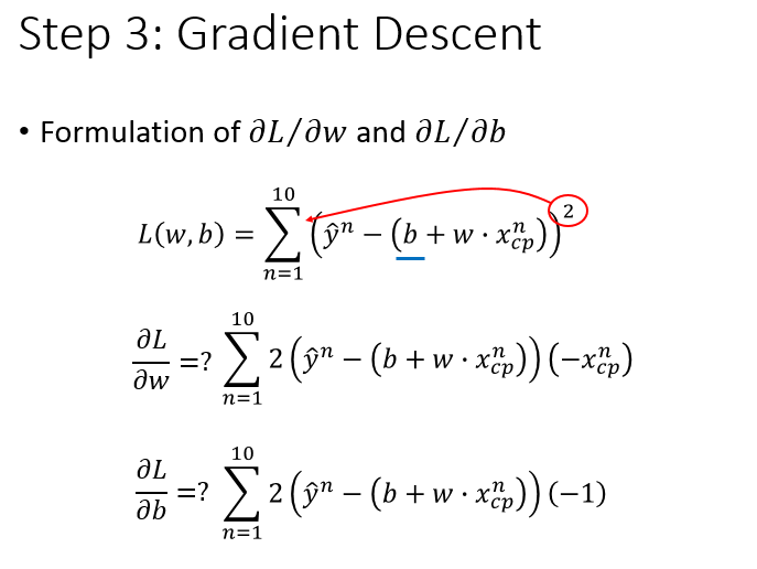
若采用方差来评估，则 L(w, b) = \(\sum_{n=1}^{10}(\hat{y}^n-(b+{w·x_{cp}}^n))^{2}\)

（其中，\(\hat{y}\): 表示正确的，实际观测到的结果）

Step 3: Pick the Best Function

最好的函数就是使L(f)最小的函数，f* = arg \(min_f\)L(f)
w*, b* = arg \(min_{w,b}\)L(w, b) = arg \(min_{w, b}\)\(\sum_{n=1}^{10}(\hat{y}^n-(b+{w·x_{cp}}^n))^{2}\)

如何计算呢？用的就是梯度下降法，Gradient Descent,

如果只考虑 w 一个变量：

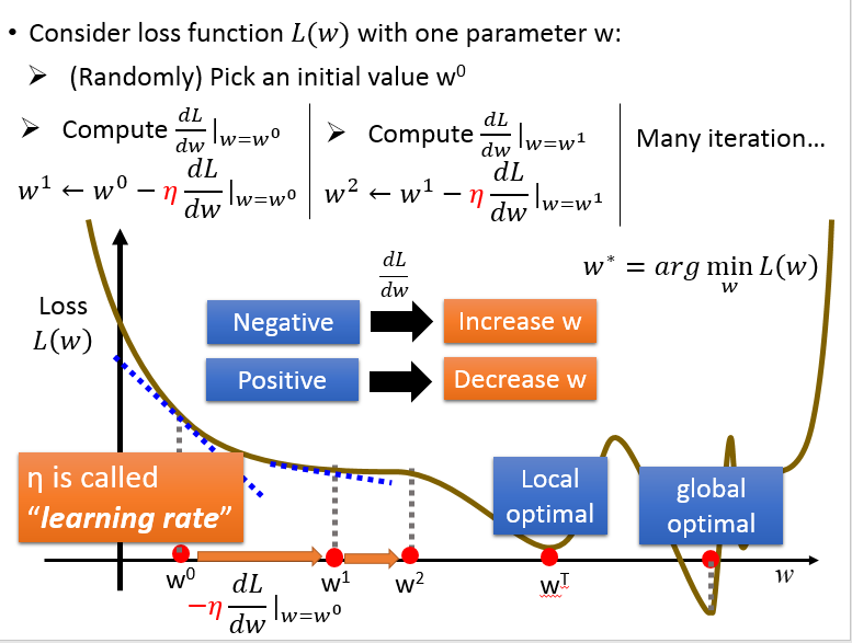
同时考虑 w, b 两个变量：

因为线性回归的损失函数总是一个凸函数，所以不用考虑局部最小，得到的就是全局最小。

对损失函数求导得到：

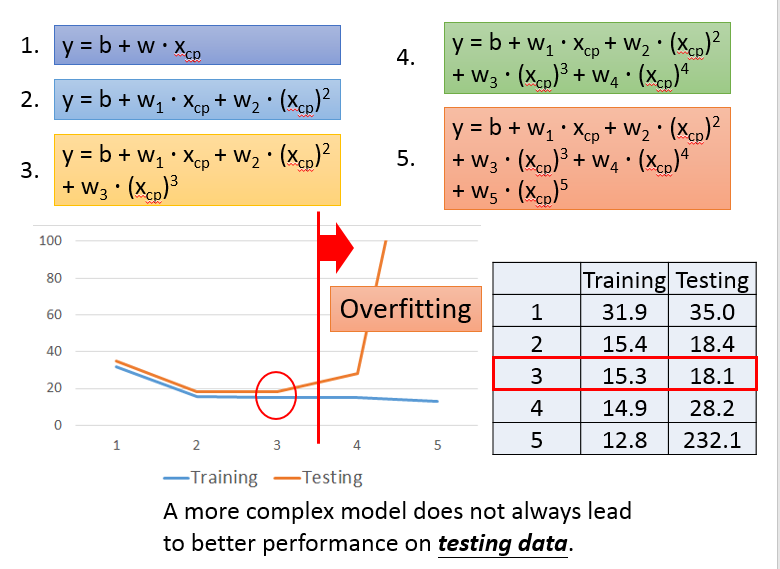
根据泰勒公式，考虑更多的项，得到如下的结果：（加了高次项依然是linear model，因为\(x_{cp}\)不是参数）

当收集到更多的数据后，会发现可能还有其他未考虑的因素，

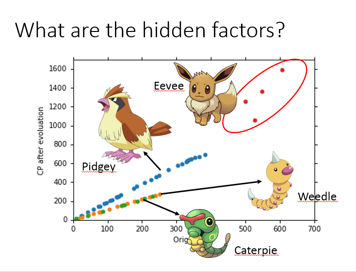
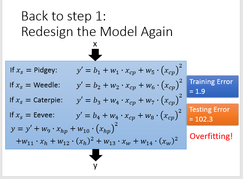
可以对模型修正为，y = \(\delta(x_s)·(b + \sum w_i x_i)\)，其中 \(\delta(x_s)\) 的取值是二元的。

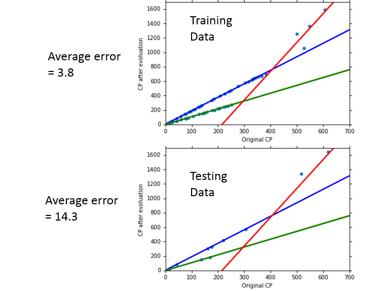
可以看到拟合的效果更好了，但是如果考虑的因素过多，则可能也会出现 Overfitting 的问题。

最后，还需要对损失函数做正则化操作，以使其在测试数据上表现更好。

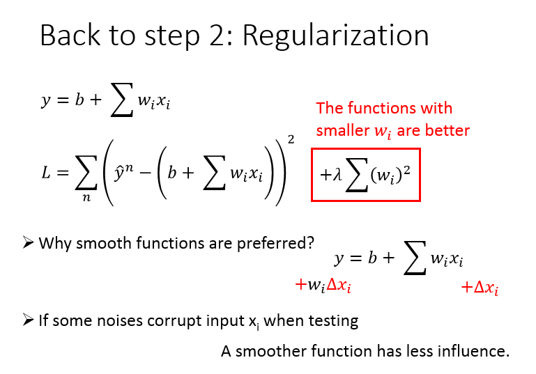
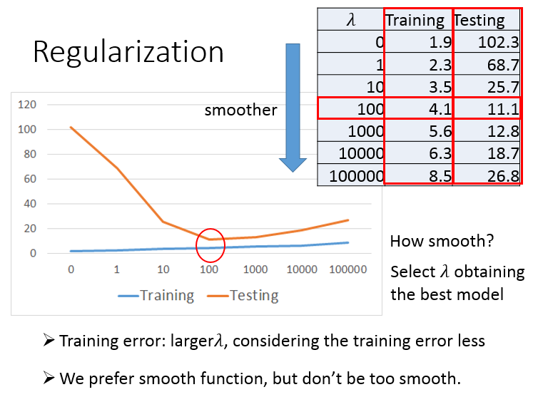
调参数 \(\lambda\)，\(\lambda\) 越大，曲线越平滑，对noise不那么敏感。
但是 \(\lambda\) 本质上是惩罚项，惩罚项太大，会使得参数空间变小，最后的结果也不会很好。

Demo程序：

import numpy as np
import matplotlib.pyplot as plt
from tqdm import tqdm_notebook

y_data, x_data -> \(\hat{y}\) 和 \(x_{cp}\) 值向量

x_data = [338.,333.,328.,207.,226.,25.,170.,60.,208.,606.]
y_data = [640.,633.,619.,393.,428.,27.,193.,66.,226.,1591.]
# ydata = b + w * xdata

x, y -> bias, weight

x = np.arange(-200, -100, 1)
y = np.arange(-5, 5, 0.1)
X, Y = np.meshgrid(x, y)

z -> L(w, b)

z = np.zeros((len(x), len(y)))

for i in range(len(x)):
    for j in range(len(y)):
        b = x[i]
        w = y[j]
        z[j][i] = 0
        for n in range(len(x_data)):
            z[j][i] = z[j][i] + (y_data[n] - b - w*x_data[n])**2
        z[j][i] = z[j][i] / len(x_data)

b = -120 # initial b
w = -4   # initial w
lr = 1 # learning rate
iteration = 1000000

# store initial value for plotting
b_history = [b]
w_history = [w]

lr_b = 0
lr_w = 0

# iteration
for i in tqdm_notebook(range(iteration)):
    b_grad = 0.0
    w_grad = 0.0
    
    for n in range(len(x_data)):
        b_grad = b_grad - 2.0*(y_data[n] - b - w*x_data[n])*1.0
        w_grad = w_grad - 2.0*(y_data[n] - b - w*x_data[n])*x_data[n]
    
    # AdaGrad
    lr_b = lr_b + b_grad ** 2
    lr_w = lr_w + w_grad ** 2
    
    # update parameters
    b = b - lr/np.sqrt(lr_b) * b_grad
    w = w - lr/np.sqrt(lr_w) * w_grad
    
    # b = b - lr*b_grad
    # w = w - lr*w_grad
    
    # store parameters for plotting
    b_history.append(b)
    w_history.append(w)

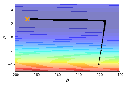
# plot the figure
plt.contourf(x, y, z, 50, alpha=0.5, cmap=plt.get_cmap('jet'))
plt.plot([-188.4], [2.67], 'x', ms=12, markeredgewidth=3, color='orange')
plt.plot(b_history, w_history, 'o-', ms=3, lw=1.5, color='black')
plt.xlim(-200, -100)
plt.ylim(-5, 5)
plt.xlabel(r'$b$', fontsize=16)
plt.ylabel(r'$w$', fontsize=16)
plt.show()