

目标检测---SSD
本文转自:
https://blog.csdn.net/thisiszdy/article/details/89576389
SSD原理解读-从入门到精通
https://blog.csdn.net/qianqing13579/article/details/82106664
目标检测中anchor那些事(一)
https://blog.csdn.net/weixin_45209433/article/details/104972124
SSD: Single Shot MultiBox Detector
论文链接:https://arxiv.org/abs/1512.02325
论文翻译:https://blog.csdn.net/denghecsdn/article/details/77429978
论文详解:https://blog.csdn.net/WZZ18191171661/article/details/79444217

1、算法步骤:
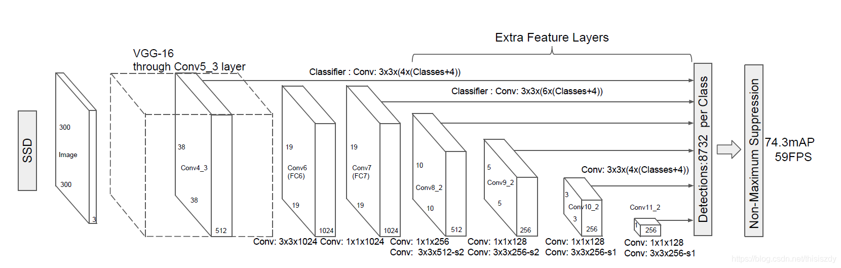
1、输入一幅图片(300x300),将其输入到预训练好的分类网络中来获得不同大小的特征映射,修改了传统的VGG16网络;
将VGG16的FC6和FC7层转化为卷积层,如图1上的Conv6和Conv7;
去掉所有的Dropout层和FC8层;
添加了Atrous算法(hole算法);
将Pool5从2x2-S2变换到3x3-S1;
2、抽取Conv4_3、Conv7、Conv8_2、Conv9_2、Conv10_2、Conv11_2层的feature map,然后分别在这些feature map层上面的每一个点构造6个不同尺度大小的bbox,然后分别进行检测和分类,生成多个bbox,如图2所示;
3、将不同feature map获得的bbox结合起来,经过NMS(非极大值抑制)方法来抑制掉一部分重叠或者不正确的bbox,生成最终的bbox集合(即检测结果);
2、算法细节
(1)多尺度特征映射
SSD算法中使用到了conv4_3,conv_7,conv8_2,conv7_2,conv8_2,conv9_2,conv10_2,conv11_2这些大小不同的feature maps,其目的是为了能够准确的检测到不同尺度的物体,因为在低层的feature map,感受野比较小,高层的感受野比较大,在不同的feature map进行卷积,可以达到多尺度的目的。
Why?:我们将一张图片输入到一个卷积神经网络中,经历了多个卷积层和池化层,我们可以看到在不同的卷积层会输出不同大小的feature map(这是由于pooling层的存在,它会将图片的尺寸变小),而且不同的feature map中含有不同的特征,而不同的特征可能对我们的检测有不同的作用。总的来说,浅层卷积层对边缘更加感兴趣,可以获得一些细节信息,而深层网络对由浅层特征构成的复杂特征更感兴趣,可以获得一些语义信息,对于检测任务而言,一幅图像中的目标有复杂的有简单的,对于简单的patch我们利用浅层网络的特征就可以将其检测出来,对于复杂的patch我们利用深层网络的特征就可以将其检测出来,因此,如果我们同时在不同的feature map上面进行目标检测,理论上面应该会获得更好的检测效果。
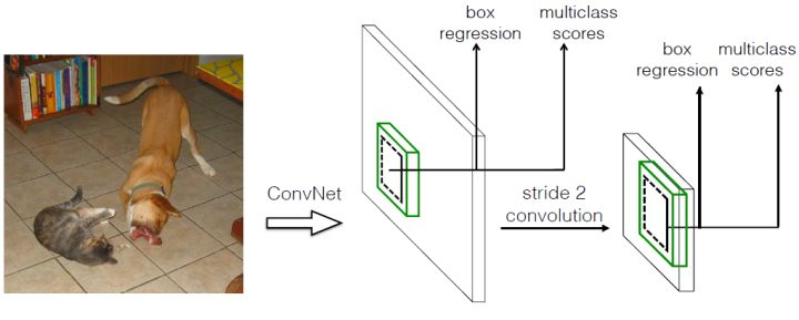
(2)Defalut box
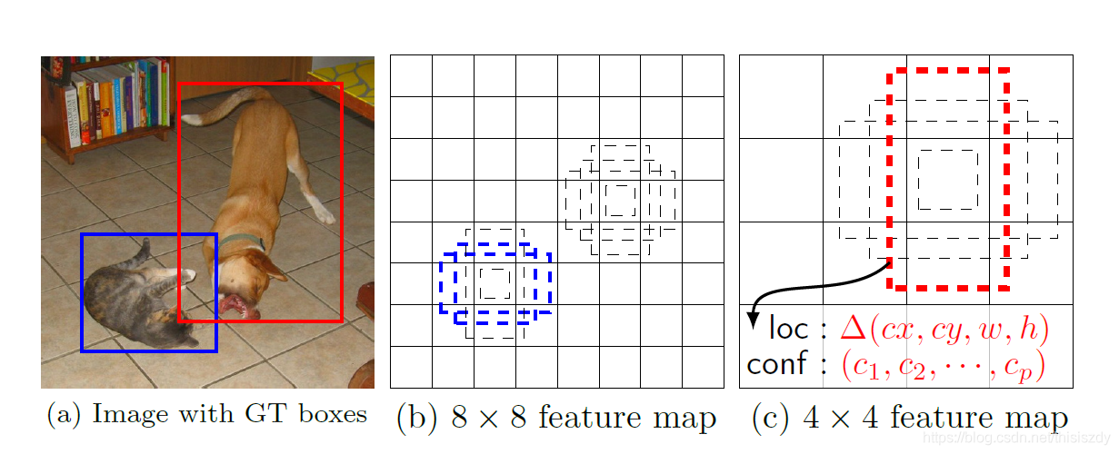
如上图所示,在特征图的每个位置预测K个bbox,对于每一个bbox,预测C个类别得分,以及相对于Default box的4个偏移量值,这样总共需要 (C+4)×K个预测器,则在m×n的feature map上面将会产生 (C+4)×K×m×n个预测值。
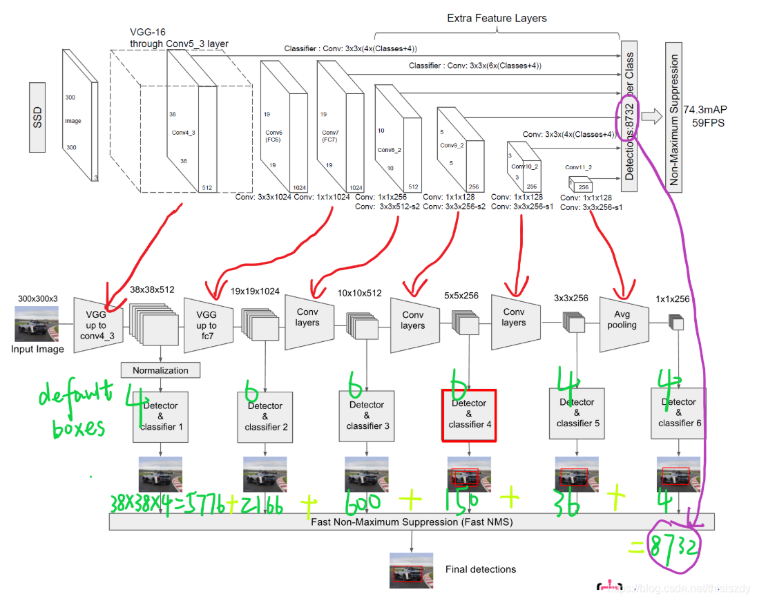
SSD中的Defalut box和Faster-rcnn中的anchor机制很相似。就是预设一些目标预选框,后续通过softmax分类+bounding box regression获得真实目标的位置。对于不同尺度的feature map 上使用不同的Default boxes。如上图所示,我们选取的feature map包括38x38x512、19x19x1024、10x10x512、5x5x256、3x3x256、1x1x256,Conv4_3之后的feature map默认的box是4个,我们在38x38的这个平面上的每一点上面获得4个box,那么我们总共可以获得38x38x4=5776个;同理,我们依次将FC7、Conv8_2、Conv9_2、Conv10_2和Conv11_2的box数量设置为6、6、6、4、4,那么我们可以获得的box分别为2166、600、150、36、4,即我们总共可以获得8732个box,然后我们将这些box送入NMS模块中,获得最终的检测结果。
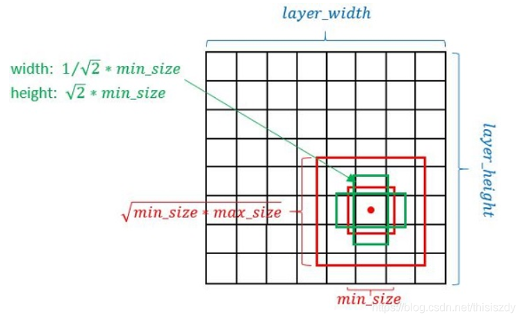
Defalut box生成规则:
以feature map上每个点的中点为中心(offset=0.5),生成一系列同心的Defalut box(然后中心点的坐标会乘以step,相当于从feature map位置映射回原图位置)
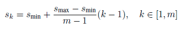
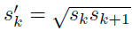
使用m(SSD300中m=6)个不同大小的feature map 来做预测,最底层的 feature map 的 scale 值为 Smin=0.2,最高层的为Smax=0.95,其他层通过下面的公式计算得到:
使用不同的ratio值,[1, 2, 3, 1/2, 1/3],通过下面的公式计算 default box 的宽度w和高度h

而对于ratio=0的情况,指定的scale如下所示,即总共有 6 中不同的 default box。
ssd基本的简洁框架
-----------分割线----------------------------
经典的代码当然值得一读再读,深挖细节,但是也是面试的时候老是被问到这些细节的东东才来下定决心研究的。
研究的是pytorch版本的ssd,由于代码比较年老,需要修改一些才能正常训练。
1.报错解决
iter 4138 || Loss: 6.2725 || Traceback (most recent call last):
  File "train.py", line 257, in <module>
    train()
  File "train.py", line 167, in train
    images, targets = next(batch_iterator)
  File "/data_1/Yang/software_install/Anaconda1105/envs/pytorch1.7/lib/python3.7/site-packages/torch/utils/data/dataloader.py", line 435, in __next__
    data = self._next_data()
  File "/data_1/Yang/software_install/Anaconda1105/envs/pytorch1.7/lib/python3.7/site-packages/torch/utils/data/dataloader.py", line 1058, in _next_data
    raise StopIteration
StopIteration
仔细分析了一下:
len_dataset_my = len(dataset) 是16551.说明是16551张图片
  data_loader = data.DataLoader(dataset, args.batch_size,
                                  num_workers=args.num_workers,
                                  shuffle=True, collate_fn=detection_collate,
                                  pin_memory=True)

    len_data_loader = len(data_loader)
len_data_loader是4138, 由于我batchsize是4, 16551/4 = 4137.75
奔溃的地方是在下面触发的
    for iteration in range(args.start_iter, cfg['max_iter']):
        if args.visdom and iteration != 0 and (iteration % epoch_size == 0):
            update_vis_plot(epoch, loc_loss, conf_loss, epoch_plot, None,
                            'append', epoch_size)
            # reset epoch loss counters
            loc_loss = 0
            conf_loss = 0
            epoch += 1

        if iteration in cfg['lr_steps']:
            step_index += 1
            adjust_learning_rate(optimizer, args.gamma, step_index)

        # load train data
        images, targets = next(batch_iterator)
因为经过4138次之后,next已经没有数据了。那么可以修改如下:
try:
     images, targets = next(batch_iterator)
except StopIteration:
     batch_iterator = iter(data_loader)
     images, targets = next(batch_iterator)
2.target = np.hstack((boxes, np.expand_dims(labels, axis=1)))
boxes 是ndarray [2,4]
labels 是ndarray [2,]
然后target = np.hstack((boxes, np.expand_dims(labels, axis=1)))
target就是ndarray [2,5]
3.itertools.product
在ssd代码中prior_box.py有段代码这么写:
        from itertools import product as product
        for k, f in enumerate(self.feature_maps): #[38, 19, 10, 5, 3, 1],
            for i, j in product(range(f), repeat=2):
                f_k = self.image_size / self.steps[k]
                ...
product(A,B)函数,返回A和B中的元素组成的笛卡尔积的元组
import itertools
for item in itertools.product([1,2,3,4],[100,200]):
    print(item)
    '''
(1, 100)
(1, 200)
(2, 100)
(2, 200)
(3, 100)
(3, 200)
(4, 100)
(4, 200)
    '''
product 用于求多个可迭代对象的笛卡尔积(Cartesian Product),它跟嵌套的 for 循环等价.即:
product(A, B) 和 ((x,y) for x in A for y in B)一样.
它的一般使用形式如下:
itertools.product(*iterables, repeat=1)
iterables是可迭代对象,repeat指定iterable重复几次,即:
product(A,repeat=3)等价于product(A,A,A)
import itertools

feature_maps = [6, 5, 4, 3, 2, 1]
for k, f in enumerate(feature_maps):  # [38, 19, 10, 5, 3, 1],
    for i, j in itertools.product(range(f), repeat=2):
        print(i,j)
0 0
0 1
0 2
0 3
0 4
0 5
1 0
1 1
1 2
1 3
1 4
1 5
2 0
2 1
2 2
2 3
2 4
2 5
4.矩阵下标操作
4.1
truths = targets[idx][:, :-1].data
labels = targets[idx][:, -1].data
targets[idx]比如是[6,5], 5表示的是xmin,ymin,xmax,ymax,label
所以truths表示坐标取前4位。targets[idx][:, :-1]
而label只需要取最后一位就可以。targets[idx][:, -1]
4.2
def point_form(boxes):
    """ Convert prior_boxes to (xmin, ymin, xmax, ymax)
    representation for comparison to point form ground truth data.
    Args:
        boxes: (tensor) center-size default boxes from priorbox layers.
    Return:
        boxes: (tensor) Converted xmin, ymin, xmax, ymax form of boxes.
    """
    return torch.cat((boxes[:, :2] - boxes[:, 2:]/2,     # xmin, ymin
                     boxes[:, :2] + boxes[:, 2:]/2), 1)  # xmax, ymax
boxes是anchor,大小是[8732,4],格式是cx,cy,w,h
boxes[:, :2] - boxes[:, 2:]/2 -->>[8732,2]
boxes[:, :2] + boxes[:, 2:]/2 -->>[8732,2]
torch.cat((boxes[:, :2] - boxes[:, 2:]/2,boxes[:, :2] + boxes[:, 2:]/2), 1) -->[8732,4]
4.3
def intersect(box_a, box_b):
    """ We resize both tensors to [A,B,2] without new malloc:
    [A,2] -> [A,1,2] -> [A,B,2]
    [B,2] -> [1,B,2] -> [A,B,2]
    Then we compute the area of intersect between box_a and box_b.
    Args:
      box_a: (tensor) bounding boxes, Shape: [A,4].
      box_b: (tensor) bounding boxes, Shape: [B,4].
    Return:
      (tensor) intersection area, Shape: [A,B].
    """
    A = box_a.size(0)
    B = box_b.size(0)
    max_xy = torch.min(box_a[:, 2:].unsqueeze(1).expand(A, B, 2),
                       box_b[:, 2:].unsqueeze(0).expand(A, B, 2))
    min_xy = torch.max(box_a[:, :2].unsqueeze(1).expand(A, B, 2),
                       box_b[:, :2].unsqueeze(0).expand(A, B, 2))
    inter = torch.clamp((max_xy - min_xy), min=0)
    return inter[:, :, 0] * inter[:, :, 1]
box_a 是[A,4]
box_b 是[B,4],B=8732
box_a是groundtruth的矩形框,这个函数目的就是把A个框与每个anchor计算交并比。所以,挨个剖析每一句:
def intersect(box_a, box_b):
""" We resize both tensors to [A,B,2] without new malloc:
    [A,2] -> [A,1,2] -> [A,B,2]
    [B,2] -> [1,B,2] -> [A,B,2]
    Then we compute the area of intersect between box_a and box_b.
    Args:
      box_a: (tensor) bounding boxes, Shape: [A,4].
      box_b: (tensor) bounding boxes, Shape: [B,4].
    Return:
      (tensor) intersection area, Shape: [A,B].
box_a [2,4]
box_b [8732,4]
 """
    A = box_a.size(0) #2
    B = box_b.size(0) #8732

    n1 = box_a[:, 2:] #[2,2]
    n1_1 = box_a[:, 2:].unsqueeze(1) #[2,1,2]
    n1_2 = box_a[:, 2:].unsqueeze(1).expand(A, B, 2) #[2,8732,2]  这里是每个pt复制了8732个

    n2 = box_b[:, 2:] #[8732,2]
    n2_1 = box_b[:, 2:].unsqueeze(0) #[1,8732,2]
    n2_2 = box_b[:, 2:].unsqueeze(0).expand(A, B, 2) #[2,8732,2]

    n3 = torch.min(n1_2, n2_2) #[2,8732,2] ## 计算了每个groundtruth的pt_br的坐标与每个anchor的最小点坐标

    max_xy = torch.min(box_a[:, 2:].unsqueeze(1).expand(A, B, 2),
                       box_b[:, 2:].unsqueeze(0).expand(A, B, 2)) ## 计算了每个groundtruth的pt_br的坐标与每个anchor的最小点坐标
    min_xy = torch.max(box_a[:, :2].unsqueeze(1).expand(A, B, 2),
                       box_b[:, :2].unsqueeze(0).expand(A, B, 2))## 计算了每个groundtruth的pt_tl的坐标与每个anchor的最大点坐标
    sub_ = max_xy - min_xy #[2,8732,2] 相交区域的长与宽
    inter = torch.clamp((max_xy - min_xy), min=0) #负数截断为0
    return inter[:, :, 0] * inter[:, :, 1] #[2,8732] 每个gt与每个anchor相交区域的面积
这段代码很厉害,不用for循环就可以计算出每个gt与8732个anchor之间的交并比。
4.4 torch.max
torch.max的用法
(max, max_indices) = torch.max(input, dim, keepdim=False)

    输入:
    1、input 是输入的tensor。
    2、dim 是索引的维度,dim=0寻找每一列的最大值,dim=1寻找每一行的最大值。
    3、keepdim 表示是否需要保持输出的维度与输入一样,keepdim=True表示输出和输入的维度一样,keepdim=False表示输出的维度被压缩了,也就是输出会比输入低一个维度。
    输出:
    1、max 表示取最大值后的结果。
    2、max_indices 表示最大值的索引。
先看keepdim=True,False的效果
import torch
x = torch.randint(0,9,(2,4))
print("x=")
print(x)

a1_val,a1_index = x.max(1, keepdim=True)
a11_val,a11_index = x.max(1, keepdim=False)

print("a1=")
print(a1_val)
print(a1_val.shape)
print(a1_index)

print("a11=")
print(a11_val)
print(a11_val.shape)
print(a11_index)
x=
tensor([[5, 2, 4, 1],
        [7, 0, 8, 6]])
a1=
tensor([[5],
        [8]])
torch.Size([2, 1])
tensor([[0],
        [2]])
a11=
tensor([5, 8])
torch.Size([2])
tensor([0, 2])

Process finished with exit code 0
可以看到,keepdim=True的时候,原来的shape是[2,4],然后max之后的val是[2, 1]。可见维度是不变的。
再看dim=0,1
import torch
x = torch.randint(0,9,(2,4))
print("x=")
print(x)
a1_val,a1_index = x.max(1, keepdim=True)
a2_val,a2_index = x.max(0, keepdim=True)
print("a1=")
print(a1_val)
print(a1_val.shape)
print(a1_index)

print("a2=")
print(a2_val)
print(a2_val.shape)
print(a2_index)
x=
tensor([[0, 6, 5, 4],
        [5, 5, 7, 6]])
a1=
tensor([[6],
        [7]])
torch.Size([2, 1])
tensor([[1],
        [2]])
a2=
tensor([[5, 6, 7, 6]])
torch.Size([1, 4])
tensor([[1, 0, 1, 1]])
dim=1,是按照行来的
dim=0,是按照列来的
4.5 下表索引
import torch
x = torch.randint(0,9,(10,2))
print("x=")
print(x)
print("---"*8)


idx = torch.randint(0,9,(4,1)).squeeze()
print("idx=")
print(idx)
print("---"*8)

x_selete = x[idx]
print(x_selete)
x=
tensor([[7, 6],
        [6, 7],
        [5, 4],
        [1, 8],
        [8, 6],
        [4, 6],
        [5, 5],
        [2, 0],
        [1, 5],
        [8, 7]])
------------------------
idx=
tensor([8, 1, 8, 6])
------------------------
tensor([[1, 5],
        [6, 7],
        [1, 5],
        [5, 5]])
对应源码里面是
matches = truths[best_truth_idx]
所以,这里的语法很精简,就是和Python类似。
a = b[c]
比如b的shape是[5,4]
c的shape是[100],c的取值范围是0-5.那么就是按照c的索引取b的值。
4.6 pytorch sort, 两次sort操作
import torch

x = torch.randn((4,5))

_,indices = x.sort(dim=1,descending=True)

_,idx = indices.sort(dim=1)

print(x)
print()
print(idx)

aa = idx < 2
print(aa)

x_selete = x[aa]
print(x_selete)
# x
tensor([[ 0.2667,  0.8747,  0.2998, -0.2021,  2.3771],
        [ 1.0459, -0.0745, -1.2888, -0.0867, -0.4641],
        [ 0.0052, -2.1177, -0.7523,  1.9897, -0.9098],
        [ 0.0294, -1.0081, -0.8528, -0.4864, -0.7573]])

#idx
tensor([[3, 1, 2, 4, 0],
        [0, 1, 4, 2, 3],
        [1, 4, 2, 0, 3],
        [0, 4, 3, 1, 2]])
这里可以分析其结果。就是每一行,对应的是x降续的下标。比如拿第一行举例:
0.2667,  0.8747,  0.2998, -0.2021,  2.3771
3,          1,       2,      4,        0
就是0代表最大,1,2,后面其次。
这种做法就是相当于保持坐标位置不变,每个值都对应排序的结果。

#aa
tensor([[False,  True, False, False,  True],
        [ True,  True, False, False, False],
        [ True, False, False,  True, False],
        [ True, False, False,  True, False]])
aa = idx < 2
这个意思就是取出最大值的前2位。这样得到的坐标也和x一样的格式,每行值前2位是true,其余false

#x_selete  x_selete = x[aa]对应是true的位置的元素取出来
tensor([ 0.8747,  2.3771,  1.0459, -0.0745,  0.0052,  1.9897,  0.0294, -0.4864])

 浙公网安备 33010602011771号