实验一 感知器及其应用

博客班级	机器学习
作业要求	要求
作业目标	感知器算法的理解及应用
学号	3180701213

一.实验目的

1.理解感知器算法原理，能实现感知器算法；

2.掌握机器学习算法的度量指标；

3.掌握最小二乘法进行参数估计基本原理；

4.针对特定应用场景及数据，能构建感知器模型并进行预测。

二.实验内容

1.安装Pycharm，注册学生版。

2.安装常见的机器学习库，如Scipy、Numpy、Pandas、Matplotlib，sklearn等。

3.编程实现感知器算法。

4.熟悉iris数据集，并能使用感知器算法对该数据集构建模型并应用

三.实验过程及结果

实验代码及注释

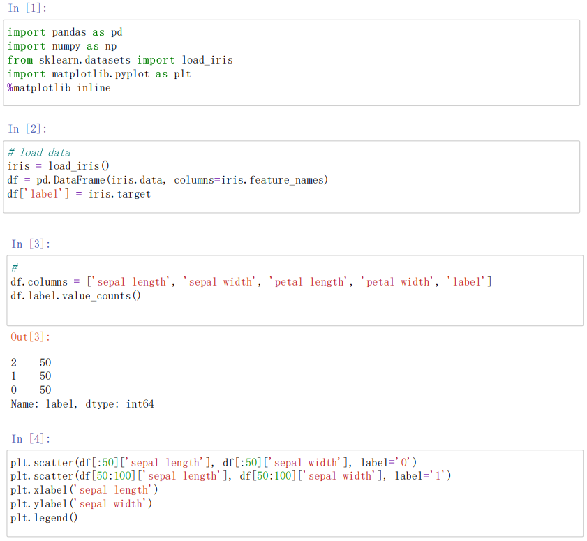
//导入pandas/numpy/matplotlib/sklearn机器学习库
import pandas as pd
import numpy as np
//导入iris数据集
from sklearn.datasets import load_iris
import matplotlib.pyplot as plt
%matplotlib inline

#load data
iris=load_iris()  //这里是sklearn中自带的一部分数据
df=pd.DataFrame(iris.data,columns=iris.feature_names)  ////将列名设置为特征
df['label'] = iris.target  //增加一列为类别标签

df.columns = ['sepal length', 'sepal width', 'petal length', 'petal width', 'label']//将各个列重命名
df.label.value_counts()value_counts//确认数据出现的频率

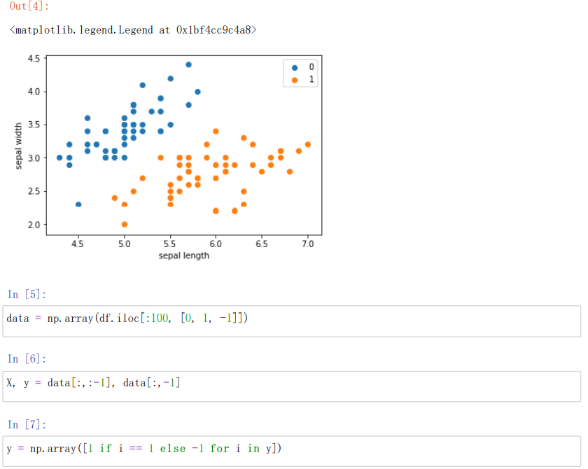
#画散点图，第一维数据作为x轴，第二维数据作为y轴，['sepal length'，'sepal width']特征分布查看
plt.scatter(df[:50]['sepal length'], df[:50]['sepal width'], label='0')  //绘制散点图
plt.scatter(df[50:100]['sepal length'], df[50:100]['sepal width'], label='1')
plt.xlabel('sepal length')  
plt.ylabel('sepal width')
plt.legend()

data = np.array(df.iloc[:100, [0, 1, -1]])按行索引,取出第0，1，-1列

X, y = data[:,:-1], data[:,-1]//X为sepal length，sepal width y为标签

y = np.array([1 if i == 1 else -1 for i in y])将两个类别设重新设置为+1 —1

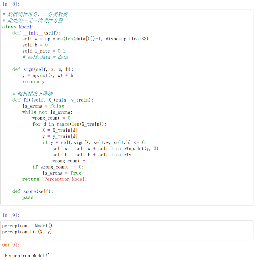
#数据线性可分，二分类数据
#此处为一元一次线性方程
class Model:
def init(self):  //将参数w1,w2置为1 b置为0 学习率为0.1
self.w = np.ones(len(data[0])-1, dtype=np.float32)  //data[0]为第一行的数据len（data[0]=3)这里取两个w权重参数
self.b = 0
self.l_rate = 0.1
%# self.data = data
def sign(self, x, w, b):
y = np.dot(x, w) + b
return y
#随机梯度下降法
def fit(self, X_train, y_train):  //拟合训练数据求w和b
is_wrong = False  //判断是否误分类
while not is_wrong:
wrong_count = 0
for d in range(len(X_train)):  //取出样例，不断的迭代
X = X_train[d]
y = y_train[d]
if y * self.sign(X, self.w, self.b) <= 0:  //根据错误的样本点不断的更新和迭代w和b的值（根据相乘结果是否为负来判断是否出错，本题将0也归为错误）
self.w = self.w + self.l_ratenp.dot(y, X)
self.b = self.b + self.l_ratey
wrong_count += 1
if wrong_count == 0:  //直到误分类点为0 跳出循环
is_wrong = True
return 'Perceptron Model!'

def score(self):
pass

perceptron = Model()
perceptron.fit(X, y)//感知机模型

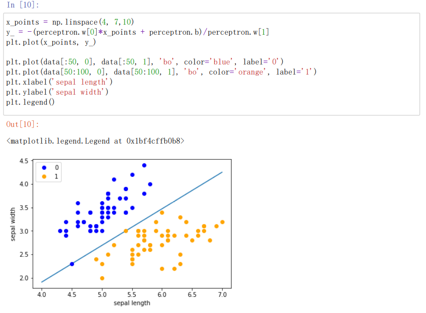
#绘制模型图像，定义一些基本的信息
x_points = np.linspace(4, 7,10)  //x轴的划分
y_ = -(perceptron.w[0]*x_points + perceptron.b)/perceptron.w[1]
plt.plot(x_points, y_)  //绘制模型图像（数据、颜色、图例等信息）
plt.plot(data[:50, 0], data[:50, 1], 'bo', color='blue', label='0')
plt.plot(data[50:100, 0], data[50:100, 1], 'bo', color='orange', label='1')
plt.xlabel('sepal length')
plt.ylabel('sepal width')
plt.legend()

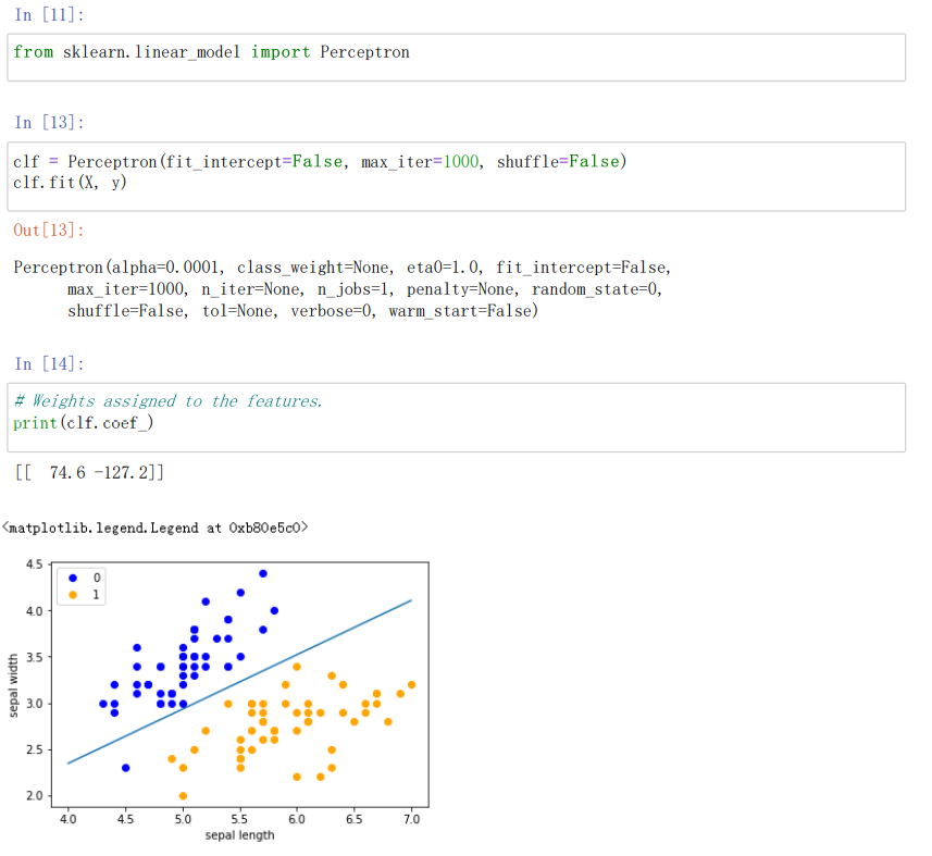
from sklearn.linear_model import Perceptron//定义感知机（下面将使用感知机）

clf = Perceptron(fit_intercept=False, max_iter=1000, shuffle=False)
clf.fit(X, y)//使用训练数据拟合

%# Weights assigned to the features.
print(clf.coef_)//输出感知机模型参数

%# 截距 Constants in decision function.
print(clf.intercept_)//输出感知机模型参数

x_ponits = np.arange(4, 8)  //确定x轴和y轴的值
y_ = -(clf.coef_[0][0]*x_ponits + clf.intercept_)/clf.coef_[0][1]
plt.plot(x_ponits, y_)  //确定拟合的图像的具体信息（数据点，线，大小，粗细颜色等内容）
plt.plot(data[:50, 0], data[:50, 1], 'bo', color='blue', label='0')
plt.plot(data[50:100, 0], data[50:100, 1], 'bo', color='orange', label='1')
plt.xlabel('sepal length')
plt.ylabel('sepal width')
plt.legend()

实验结果截图

四.作业小结

1.psp表格

psp2.1	任务内容	计划完成需要的时间	实际完成需要的时间
planning	计划	15	14
estimate	估计这个任务需要多少时间，并规划大致工作步骤	15	30
development	开发	20	25
analysis	需求分析	16	8
design spec	生成设计文档	21	12
design review	设计复审	6	5
coding standard	代码规范	5	3
design	具体设计	10	16
coding	具体编码	35	37
code review	代码复审	6	8
test	测试	10	6
reporting	报告	6	8
test reporting	测试报告	3	2
size measurement	计算工作量	3	2
postmortem & process improvement plan	总结并提出改进计划	5	8

2.心得经验

通过本次实验我知道了安装常见的机器学习库，如Scipy、Numpy、Pandas、Matplotlib，sklearn等。通过编程实现了感知器算法，掌握了最小二乘法进行参数估计的基本原理。
通过Python语言完成了这次实验，也学会了用Python语言去画图描述数据。同时还熟悉了iris数据集，能使用感知器算法对该数据集构建模型并应用。