强化学习SQL算法（soft q learning）—— SVGD的实现（Stein Variational Gradient Descent: A General Purpose Bayesian Inference Algorithm）

代码实现地址：

https://openi.pcl.ac.cn/devilmaycry812839668/softlearning/src/branch/master/softlearning/misc/kernel.py

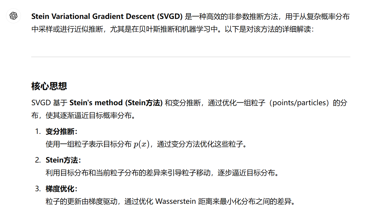
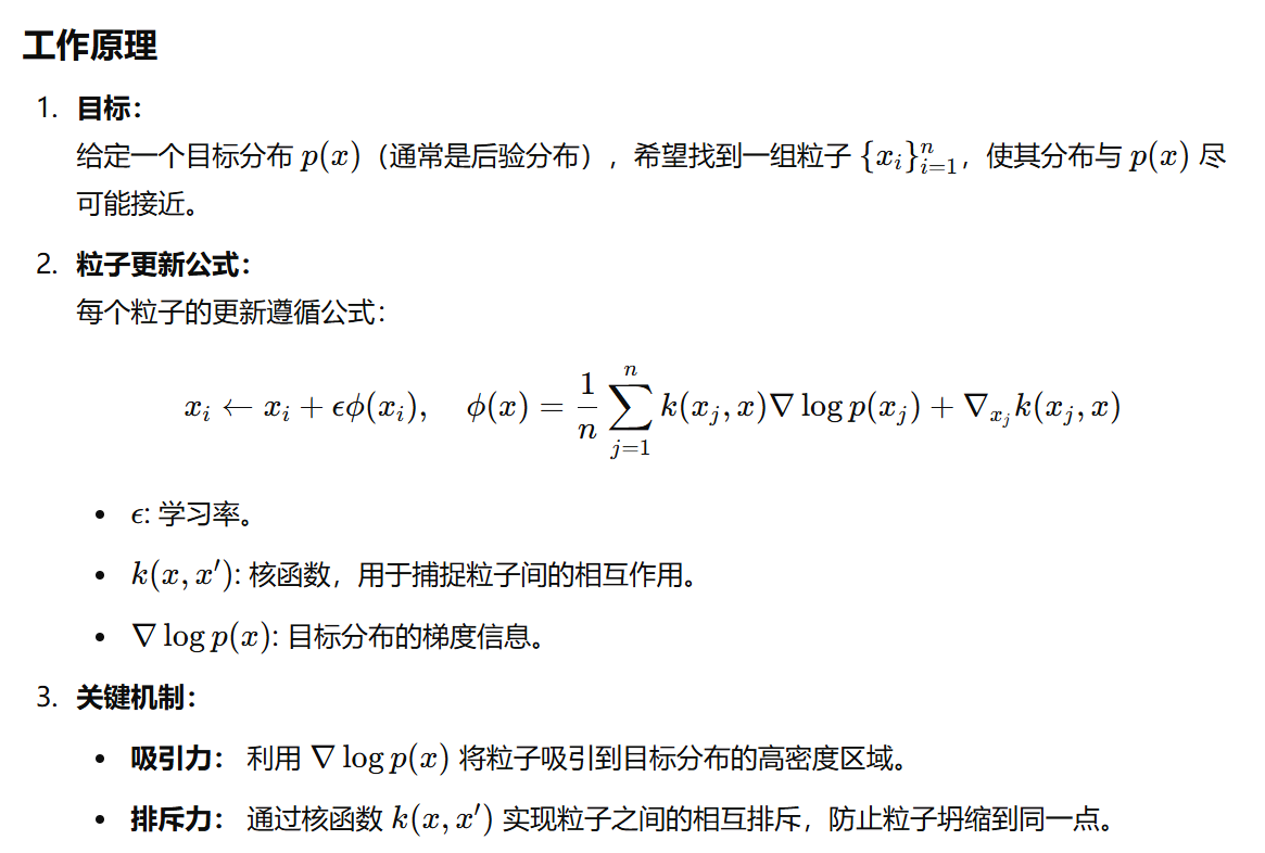
SVGD 是一种高效、灵活的推断方法，尤其适合高维度复杂分布的近似问题。

from distutils.version import LooseVersion

import numpy as np
import tensorflow as tf


def adaptive_isotropic_gaussian_kernel(xs, ys, h_min=1e-3):
    """Gaussian kernel with dynamic bandwidth.

    The bandwidth is adjusted dynamically to match median_distance / log(Kx).
    See [2] for more information.

    Args:
        xs(`tf.Tensor`): A tensor of shape (N x Kx x D) containing N sets of Kx
            particles of dimension D. This is the first kernel argument.
        ys(`tf.Tensor`): A tensor of shape (N x Ky x D) containing N sets of Kx
            particles of dimension D. This is the second kernel argument.
        h_min(`float`): Minimum bandwidth.

    Returns:
        `dict`: Returned dictionary has two fields:
            'output': A `tf.Tensor` object of shape (N x Kx x Ky) representing
                the kernel matrix for inputs `xs` and `ys`.
            'gradient': A 'tf.Tensor` object of shape (N x Kx x Ky x D)
                representing the gradient of the kernel with respect to `xs`.

    Reference:
        [2] Qiang Liu,Dilin Wang, "Stein Variational Gradient Descent: A General
            Purpose Bayesian Inference Algorithm," Neural Information Processing
            Systems (NIPS), 2016.
    """
    Kx, D = xs.get_shape().as_list()[-2:]
    Ky, D2 = ys.get_shape().as_list()[-2:]
    assert D == D2

    leading_shape = tf.shape(input=xs)[:-2]

    # Compute the pairwise distances of left and right particles.
    diff = tf.expand_dims(xs, -2) - tf.expand_dims(ys, -3)
    # ... x Kx x Ky x D

    if LooseVersion(tf.__version__) <= LooseVersion('1.5.0'):
        dist_sq = tf.reduce_sum(input_tensor=diff**2, axis=-1, keepdims=False)
    else:
        dist_sq = tf.reduce_sum(input_tensor=diff**2, axis=-1, keepdims=False)
    # ... x Kx x Ky

    # Get median.
    input_shape = tf.concat((leading_shape, [Kx * Ky]), axis=0)
    values, _ = tf.nn.top_k(
        input=tf.reshape(dist_sq, input_shape),
        k=(Kx * Ky // 2 + 1),  # This is exactly true only if Kx*Ky is odd.
        sorted=True)  # ... x floor(Ks*Kd/2)

    medians_sq = values[..., -1]  # ... (shape) (last element is the median)

    h = medians_sq / np.log(Kx)  # ... (shape)
    h = tf.maximum(h, h_min)
    h = tf.stop_gradient(h)  # Just in case.
    h_expanded_twice = tf.expand_dims(tf.expand_dims(h, -1), -1)
    # ... x 1 x 1

    kappa = tf.exp(-dist_sq / h_expanded_twice)  # ... x Kx x Ky

    # Construct the gradient
    h_expanded_thrice = tf.expand_dims(h_expanded_twice, -1)
    # ... x 1 x 1 x 1
    kappa_expanded = tf.expand_dims(kappa, -1)  # ... x Kx x Ky x 1

    kappa_grad = -2 * diff / h_expanded_thrice * kappa_expanded
    # ... x Kx x Ky x D

    return {"output": kappa, "gradient": kappa_grad}

以下内容为ChatGPT自动生成，可靠性未验证，因此只作为参考之用：

下面的SVGD的计算方法和代码实现已经经过验证，真实可行。

代码实现（简单版本的实现）：

import numpy as np
from scipy.stats import multivariate_normal

# 核函数（RBF kernel）
def rbf_kernel(x, y, h):
    diff = x[:, None] - y[None, :]
    return np.exp(-np.sum(diff**2, axis=2) / (2 * h))

# SVGD 更新步骤
def svgd_update(particles, grad_log_p, kernel_fn, learning_rate=0.01):
    n = len(particles)
    kernel_matrix = kernel_fn(particles, particles)
    grad_kernel = -np.sum(kernel_matrix[:, :, None] * (particles[:, None] - particles[None, :]), axis=0) / len(particles)
    grad_log = grad_log_p(particles)
    update = (kernel_matrix @ grad_log + grad_kernel) / n
    particles += learning_rate * update
    return particles

# 示例目标分布：二维高斯分布
def target_grad(x):
    mean = np.array([0, 0])
    cov = np.eye(2)
    return -np.dot((x - mean), np.linalg.inv(cov))

# 初始化粒子
particles = np.random.randn(100, 2)

# 迭代更新
for _ in range(100):
    particles = svgd_update(particles, target_grad, lambda x, y: rbf_kernel(x, y, h=0.5))

print("Updated particles:", particles)

上面实现的目标分布的多维独立高斯分布均值为（0, 0），为了更明显些，修改为（10， 20），给出修改后的代码和运行结果：

import numpy as np
from scipy.stats import multivariate_normal

# 核函数（RBF kernel）
def rbf_kernel(x, y, h):
    diff = x[:, None] - y[None, :]
    return np.exp(-np.sum(diff**2, axis=2) / (2 * h))

# SVGD 更新步骤
def svgd_update(particles, grad_log_p, kernel_fn, learning_rate=0.01):
    n = len(particles)
    kernel_matrix = kernel_fn(particles, particles)
    grad_kernel = -np.sum(kernel_matrix[:, :, None] * (particles[:, None] - particles[None, :]), axis=0) / len(particles)
    grad_log = grad_log_p(particles)
    update = (kernel_matrix @ grad_log + grad_kernel) / n
    particles += learning_rate * update
    return particles

# 示例目标分布：二维高斯分布
def target_grad(x):
    mean = np.array([10, 20])
    cov = np.eye(2)
    return -np.dot((x - mean), np.linalg.inv(cov))

# 初始化粒子
particles = np.random.randn(100, 2)

# 迭代更新
for _ in range(10000):
    particles = svgd_update(particles, target_grad, lambda x, y: rbf_kernel(x, y, h=0.5))

print("Updated particles:", particles)

运行结果：