深度学习模型构建
深度学习模型构建
nn.Module
torch.nn 是 PyTorch 提供的神经网络工具包,包含了构建神经网络所需的各种组件。nn.Module 是 PyTorch 中构建神经网络的基类,所有的神经网络模型都需要继承自该类。
import torch
from torch import nn

class Model(nn.Module):                 # 神经网络Model类必须继承Module父类
    def __init__(self):                 # 初始化函数
        super(Model, self).__init__()   # 调用父类的初始化函数

    def forward(self, x):               # 前向传播
        x = nn.functional.relu(x)
        return x

model = Model()
input = torch.Tensor([1., -1.5, 2])
output = model(input)
print(output)
# tensor([1., 0., 2.])
初始化方法(__init__)中可以定义模型的各层,通常会使用如 nn.Conv2d、nn.Linear 等层组件。需要注意,调用 super(Model, self).__init__() 是必须的,它会调用父类(nn.Module)的初始化方法。
前向传播方法(forward)需要重写,定义模型的前向传播过程,说明输入数据如何经过各层处理输出结果。在前向传播过程中,可以使用激活函数(如 nn.functional.relu)或其他操作来处理数据。
PyTorch会自动通过计算图和自动微分来处理反向传播过程,无需手动编写。
卷积层
在PyTorch中,torch.nn 提供了封装好的卷积层,而 torch.nn.functional 提供了卷积函数,卷积层是对卷积函数的封装。
在卷积操作中,参数 stride 控制卷积核在输入图像上滑动的步长,可以是单一数值(统一步长)或元组(sH, sW,分别控制横向和纵向步长)。
参数 padding 在输入图像的边缘添加像素,以控制输出尺寸。padding=1 表示在图像的四周各填充一个像素,通常默认为0(不填充)。
卷积要求输入为四维张量,形状为 (batch_size, channels, height, width)。卷积核也需要是四维张量,形状为 (out_channels, in_channels, kernel_height, kernel_width)。如果尺寸不匹配,可以通过 torch.reshape() 来调整维度。
输出维度为:
import torch
from torch import nn

input = torch.tensor([[1,2,0,3,1],
                     [0,1,2,3,1],
                     [1,2,1,0,0],
                     [5,2,3,1,1],
                     [2,1,0,1,1]])

kernel = torch.tensor([[1,2,1],
                       [0,1,0],
                       [2,1,0]])

# 调整输入维度
# (batch_size, channels, height, width)
input = torch.reshape(input, (1, 1, 5, 5))
# (out_channels, in_channels, height, width)
kernel = torch.reshape(kernel, (1, 1, 3, 3))

output = nn.functional.conv2d(input, kernel,stride=1, padding=0)
print(output)
# tensor([[[[10, 12, 12],
#           [18, 16, 16],
#           [13,  9,  3]]]])
在 PyTorch 中提供了一维卷积 nn.Conv1d 处理一维数据,如时间序列信号。提供了 nn.Conv2d 处理二维数据,如图像。提供了 nn.Conv3d 处理三维数据,如视频。
卷积层可以提取图像中的局部特征(如边缘、角点等),堆叠多个卷积层能够逐渐提取更高级的特征。
卷积层的参数如下
in_channels:输入通道数。对于彩色图像,in_channels=3(RGB图像有三个通道)。out_channels:输出通道数,代表生成的卷积核数量。每个卷积核都会提取不同的特征图。kernel_size:卷积核的大小,常见为 3×3 或 5×5,决定了卷积核的感受野大小。卷积核的参数是从一些分布中进行采样得到的,在训练过程中会通过反向传播不断调整。stride:步长,控制卷积核滑动的速度。步长越大,输出的特征图越小。padding:填充,在输入数据的边缘填充额外的像素。用于控制输出的尺寸。dilation:空洞卷积,控制卷积核的“空洞”大小,增加感受野。bias:卷积层是否使用偏置项,默认是使用的。padding_mode:指定填充模式,默认是零填充。
可以利用CIFAR 10数据集训练一个简单的卷积神经网络:
import torch
from torch.utils.data import DataLoader
from torchvision import transforms, datasets
from torch.utils.tensorboard import SummaryWriter
from torch import nn

writer = SummaryWriter("logs")
transform = transforms.Compose([transforms.ToTensor()])
dataset = datasets.CIFAR10(root="Dataset", train=False, transform=transform,
                           download=True)
dataloader = DataLoader(dataset=dataset, batch_size=64, shuffle=False)

class Model(nn.Module):
    def __init__(self):
        super(Model, self).__init__()
        **self.conv = nn.Conv2d(in_channels=3, out_channels=6,
                              kernel_size=3, stride=1, padding=0)**

    def forward(self, x):
        x = self.conv(x)
        return x

model = Model()
print(model)      # 打印网络结构

step = 0
for data in dataloader:
    imgs, targets = data
    outputs = model(imgs)
    print(imgs.shape, outputs.shape)
    # 6个channel无法显示
    outputs = torch.reshape(outputs, (-1, 3, 30, 30))
    writer.add_images("Conv2d_Input", imgs, global_step=step)
    writer.add_images("Conv2d_Output", outputs, global_step=step)
    step = step + 1

writer.close()
池化层
最大池化的目的是下采样(缩小特征图),在减少数据维度的同时保留最显著的特征。从每个池化窗口中选择最大值,从而压缩空间维度,降低计算量并加速训练。
除此之外,还有上采样 MaxUnpool 、平均池化 AvgPool 等。
池化层参数如下
kernel_size:池化窗口的大小。stride:池化步幅,默认与kernel_size相同。控制池化时窗口的滑动步长。padding:是否在输入周围填充0,增加边界的输出大小。dilation:卷积核的扩张因子(通常不用于池化层)。return_indices:是否返回池化时的最大值位置,用于反向传播时的最大池化反向传播。ceil_mode:是否使用向上取整来计算池化输出的尺寸。默认为False,设置为True时,输出尺寸会向上取整。
卷积要求输入为四维张量,形状为 (batch_size, channels, height, width)。
import torch
from torch import nn

input = torch.tensor([[1, 2, 0, 3, 1],
                      [0, 1, 2, 3, 1],
                      [1, 2, 1, 0, 0],
                      [5, 2, 3, 1, 1],
                      [2, 1, 0, 1, 1]])
# 调整维度为 (batch_size, channels, height, width)
input = torch.reshape(input, shape=(1, 1, 5, 5))

class Model(nn.Module):
    def __init__(self):
        super(Model, self).__init__()
        self.pool = nn.MaxPool2d(kernel_size=3, ceil_mode=True)

    def forward(self, x):
        x = self.pool(x)
        return x

model = Model()

output = model(input)
print(output)
# tensor([[[[2, 3],
#           [5, 1]]]])
可以对CIFAR 10数据集进行一个简单的池化操作:
import torchvision.datasets
from torch import nn
from torch.utils.data import DataLoader
from torch.utils.tensorboard import SummaryWriter

writer = SummaryWriter("logs")
dataset = torchvision.datasets.CIFAR10(root="Dataset", train=False,
             **transform=torchvision.transforms.ToTensor()**, download=True)
dataloader = DataLoader(dataset, batch_size=64)

class Model(nn.Module):
    def __init__(self):
        super(Model, self).__init__()
        self.pool = nn.MaxPool2d(kernel_size=3,ceil_mode=True)

    def forward(self, x):
        x = self.pool(x)
        return x

model = Model()

step = 0
for data in dataloader:
    imgs, _ = data
    output = model(imgs)
    print(imgs.shape, output.shape)
    # torch.Size([64, 3, 32, 32]) torch.Size([64, 3, 11, 11])
    writer.add_images("pool_input", imgs, global_step=step)
    writer.add_images("pool_output", output, global_step=step)
    step = step + 1

writer.close()
非线性激活层
通过非线性激活函数,神经网络能够学习到更复杂的特征,使得模型能够拟合各种各样的函数曲线。非线性激活越多,模型的拟合能力越强。
ReLU 是最常用的非线性激活函数,它的特点是将负值全部截断为0,正值则保持不变。
参数 inplace 决定是否在原地修改输入张量。如果设置为True,则会直接修改输入数据,这样有时可以节省内存,但要小心可能会影响梯度计算。一般情况下建议 inplace=False 。
import torch
from torch import nn

input = torch.tensor([[1, -1.5],
                      [-1, 3]])

class Model(nn.Module):
    def __init__(self):
        super(Model, self).__init__()
        self.relu = nn.ReLU()

    def forward(self, x):
        x = self.relu(x)
        return x

model = Model()
output = model(input)
print(output)
# tensor([[[[1., 0.],
#           [0., 3.]]]])
对于输入矩阵中的负数,ReLU将其置为0,正数保持不变,具有一定的“稀疏性”,有助于提高模型的训练效率。
Sigmoid 函数将输入压缩到0到1之间,适合用于输出概率值。
可以对CIFAR 10数据集进行一个非线性操作:
import torchvision
from torch import nn
from torch.utils.data import DataLoader
from torch.utils.tensorboard import SummaryWriter

writer = SummaryWriter("logs")
dataset = torchvision.datasets.CIFAR10("Dataset", train=False,
                     transform=torchvision.transforms.ToTensor())
dataloader = DataLoader(dataset, batch_size=64)

# 搭建神经网络
class Model(nn.Module):
    def __init__(self):
        super(Model, self).__init__()
        self.sigmoid = nn.Sigmoid()  # inplace默认为False

    def forward(self, input):
        output = self.sigmoid(input)
        return output

model = Model()
step = 0

for data in dataloader:
    imgs, _ = data
    output = model(imgs)
    writer.add_images("Sigmoid_input", imgs, global_step=step)
    writer.add_images("Sigmoid_output", output, step)
    step = step + 1

writer.close()
线性层
Linear 层用于构建全连接层,对输入进行线性变换,将输入的特征映射到一个新的特征空间。
参数如下:
in_features:输入的特征数量(即输入的维度)。out_features:输出的特征数量(即输出的维度)。bias:是否使用偏置项,默认是True。如果设置为False,则不使用偏置。
import torch
import torch.nn as nn

class Model(nn.Module):
    def __init__(self):
        super(Model, self).__init__()
        # 全连接层
        self.linear = nn.Linear(in_features=10, out_features=5)

    def forward(self, x):
        x = self.linear(x)
        return x

# 输入维度为 (batch_size, in_features)
input = torch.randn(3, 10)

model = Model()
output = model(input)
print(output.shape)
# torch.Size([3, 5])
为了满足输入,可以采用 torch.flatten 将多维张量展平为一维张量。
参数如下:
input:要展平的输入张量。start_dim:指定展平开始的维度,默认值为0。表示从哪一维开始展平,通常start_dim=1是常见的选择(保持 batch 维度不变)。end_dim:指定展平结束的维度,默认值为-1。表示展平到哪个维度,通常将其设置为最后一维。
import torch

# (batch_size, channels, height, width)
input = torch.randn(2, 3, 4, 4)

# 使用 flatten 展平张量,start_dim=1 保持 batch_size 不变
output = torch.flatten(input, start_dim=1)

output1 = torch.flatten(input)

print(input.shape)     # torch.Size([2, 3, 4, 4])
print(output.shape)    # torch.Size([2, 48])
print(output1.shape)   # torch.Size([96])
Dropout层
torch.nn.Dropout 是一种常见的正则化方法,在训练神经网络时,通过随机丢弃神经元的激活值来防止过拟合。
torch.nn.Dropout(p=0.5, inplace=False)
其中,p 表示在每次前向传播时,随机丢弃的概率,介于 \([0,1]\)。inplace 如果设置为 True,将直接在原始输入上进行操作,而不是返回一个新的张量。
在训练模式中,Dropout 会根据 p 值随机丢弃神经元。在推理模式中,Dropout被自动禁用,网络的所有神经元都会参与计算。
因此,通常需要在模型训练时调用 model.train() 和在评估时调用 model.eval() 来切换 Dropout 的行为。
import torch
from torch import nn

# 创建一个简单的神经网络
class Model(nn.Module):
    def __init__(self):
        super(Model, self).__init__()
        self.dropout = nn.Dropout(p=0.5)  # 50% 的概率丢弃神经元

    def forward(self, x):
        x = self.dropout(x)
        return x

model = Model()

input = torch.randn(2, 5)
print(input)
# tensor([[-0.3454,  0.4890, -0.9587,  0.0146, -0.3944],
#         [ 0.2800, -1.8118, -1.4486, -3.1947, -0.6308]])

# 训练模式
model.train()
output_train = model(input)
print(output_train)
# tensor([[-0.6908,  0.0000, -0.0000,  0.0291, -0.0000],
#         [ 0.5600, -3.6236, -0.0000, -0.0000, -0.0000]])

# 评估模式
model.eval()
output_eval = model(input)
print(output_eval)
# tensor([[-0.3454,  0.4890, -0.9587,  0.0146, -0.3944],
#         [ 0.2800, -1.8118, -1.4486, -3.1947, -0.6308]])
Sequential
nn.Sequential 允许按顺序将层组合成一个模型。通过这种方式,可以更加简洁地构建网络模型。
model = nn.Sequential(
    nn.Conv2d(1, 20, 5),
    nn.ReLU(),
    nn.Conv2d(20, 64, 5),
    nn.ReLU()
)
基于 CIFAR-10,可以搭建神经网络,根绝图片内容识别属于哪一类。
神经网络首先通过卷积层提取特征,然后通过池化层降低特征维度,最后使用全连接层输出分类结果。
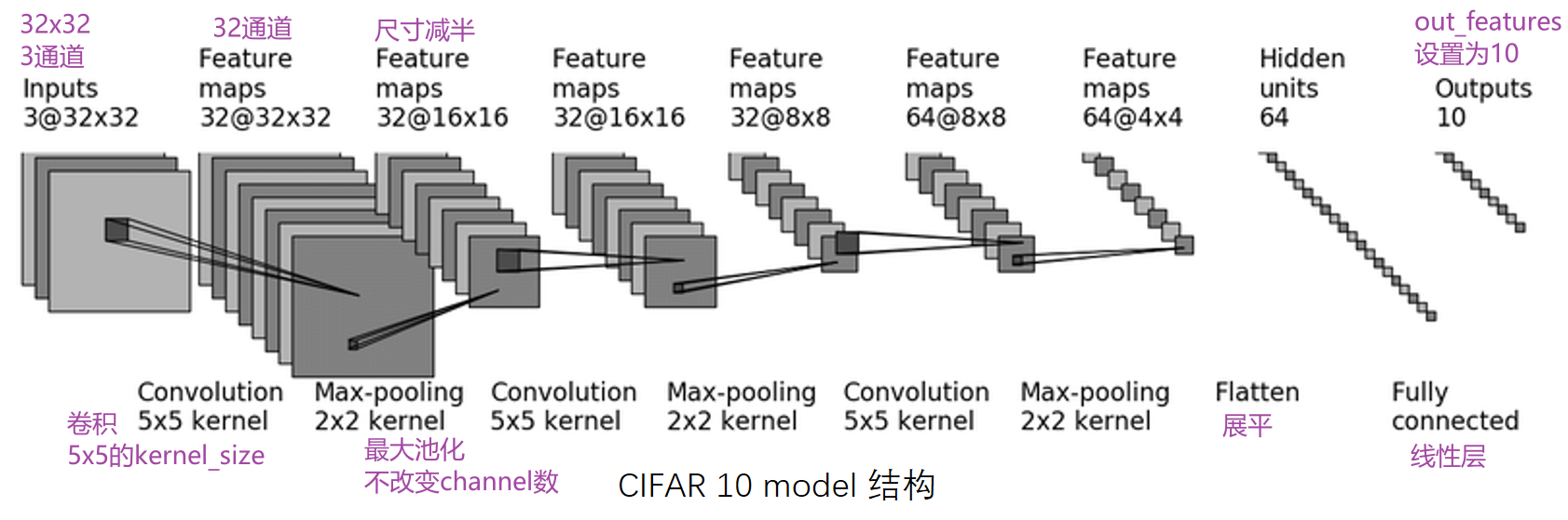
可以推测出,每次卷积的参数为 padding=2 、 stride=1 。输出的通道数等于该次卷积使用的卷积核数量。
如果不使用 Sequential ,可以采用如下代码:
import torch
from torch import nn

class Model(nn.Module):
    def __init__(self):
        super(Model, self).__init__()
        self.conv1 = nn.Conv2d(in_channels=3, out_channels=32, kernel_size=5, stride=1, padding=2)
        self.pool1 = nn.MaxPool2d(kernel_size=2)
        self.conv2 = nn.Conv2d(in_channels=32, out_channels=32, kernel_size=5, stride=1, padding=2)
        self.pool2 = nn.MaxPool2d(kernel_size=2)
        self.conv3 = nn.Conv2d(in_channels=32, out_channels=64, kernel_size=5, stride=1, padding=2)
        self.pool3 = nn.MaxPool2d(kernel_size=2)
        self.flatten = nn.Flatten()
        self.linear1 = nn.Linear(in_features=1024, out_features=64)
        self.linear2 = nn.Linear(in_features=64, out_features=10)

    def forward(self, x):
        x = self.conv1(x)
        x = self.pool1(x)
        x = self.conv2(x)
        x = self.pool2(x)
        x = self.conv3(x)
        x = self.pool3(x)
        x = self.flatten(x)     # 展平为(64, 1024)
        x = self.linear1(x)
        x = self.linear2(x)
        return x

model = Model()
print(model)

# 随机生成数据输入网络结构,看能否得到预期输出
input = torch.randn((64, 3, 32, 32))
output = model(input)
print(output.shape)
# torch.Size([64, 10])
如果使用 Sequential ,会更加方便:
import torch
from torch import nn

class Model(nn.Module):
    def __init__(self):
        super(Model, self).__init__()
        self.model1 = nn.Sequential(
            nn.Conv2d(in_channels=3, out_channels=32, kernel_size=5, stride=1, padding=2),
            nn.MaxPool2d(kernel_size=2),
            nn.Conv2d(in_channels=32, out_channels=32, kernel_size=5, stride=1, padding=2),
            nn.MaxPool2d(kernel_size=2),
            nn.Conv2d(in_channels=32, out_channels=64, kernel_size=5, stride=1, padding=2),
            nn.MaxPool2d(kernel_size=2),
            nn.Flatten(),
            nn.Linear(in_features=1024, out_features=64),
            nn.Linear(in_features=64, out_features=10)
        )

    def forward(self, x):
        x = self.model1(x)
        return x

model = Model()
print(model)
input = torch.randn((64, 3, 32, 32))
output = model(input)
print(output.shape)
# torch.Size([64, 10])
还可以通过 TensorBoard 可视化模型结构,在 TensorBoard Graph 中查看。
model = Model()
writer = SummaryWriter("logs")

input = torch.randn((64, 3, 32, 32))
writer.add_graph(model, input)

output = model(input)
writer.close()

 浙公网安备 33010602011771号