Machine Learning Algorithms Study Notes(2)--Supervised Learning

 

Machine Learning Algorithms Study Notes

 

高雪松

@雪松Cedro

Microsoft MVP

 

本系列文章是Andrew Ng 在斯坦福的机器学习课程 CS 229 的学习笔记。 

Machine Learning Algorithms Study Notes 系列文章介绍

 

2    Supervised Learning    3

2.1    Perceptron Learning Algorithm (PLA)    3

2.1.1    PLA -- "知错能改"演算法    4

2.2    Linear Regression    6

2.2.1    线性回归模型    6

2.2.2    最小二乘法( least square method)    7

2.2.3    梯度下降算法（Gradient Descent）    7

2.2.4    Spark MLlib实现线性回归    9

2.3    Classification and Logistic Regression    10

2.3.1    逻辑回归算法原理    10

2.3.2    Classifying MNIST digits using Logistic Regression    13

2.4    Softmax Regression    23

2.4.1    简介    23

2.4.2    cost function    25

2.4.3    Softmax回归模型参数化的特点    26

2.4.4    权重衰减    27

2.4.5    Softmax回归与Logistic 回归的关系    28

2.4.6    Softmax 回归 vs. k 个二元分类器    28

2.5    Generative Learning algorithms    29

2.5.1    Gaussian discriminant analysis ( GDA )    29

2.5.2    朴素贝叶斯 ( Naive Bayes )    34

2.5.3    Laplace smoothing    37

2.6    Support Vector Machines    37

2.6.1    Introduction    37

2.6.2    由逻辑回归引出SVM    38

2.6.3    function and geometric margin    40

2.6.4    optimal margin classifier    43

2.6.5    拉格朗日对偶（Lagrange duality）    44

2.6.6    optimal margin classifier revisited    46

2.6.7    Kernels    48

2.6.8    Spark MLlib -- SVM with SGD    49

2.7    神经网络    51

2.7.1    概述    51

2.7.2    神经网络模型    53

 

 

 

 

2 Supervised Learning

 

2.1 Perceptron Learning Algorithm (PLA)

Perceptron - 感知机能够根据每笔资料的特征，把资料判断为不同的类别。令 是一个perceptron，你给我一个 (是一个特征向量)，把 输入 ，它就会输出这个x  的类别，譬如在信用违约风险预测当中，输出就可能是这个人会违约，或者不会违约。本质上讲，perceptron是一种二元线性分类器，它通过对特征向量的加权求和，并与事先设定的门槛值(threshold)做比较，高于门槛值的输出1，低于门槛值的输出-1。

 

 

或者写成

 

 

 

Perceptron Learning Algorithm（感知器学习算法）的目的是要找到一个perceptron，能把正确地把不同类别的点区分开来。

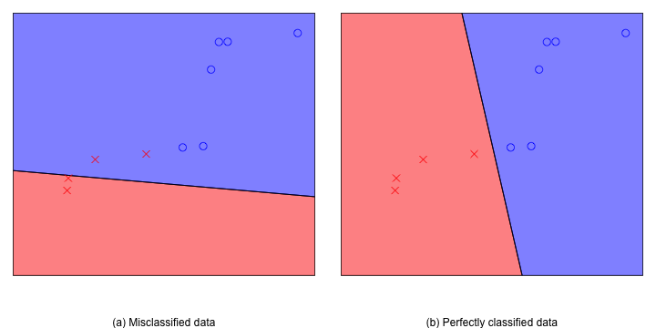
图 维空间中的两个不同的perceptron

上图中是二维平面上的两个perceptron，图中圈圈代表+1的点，叉叉代表-1的点。左边的perceptron把两个叉叉错分到圈圈当中，而右边的则很完美地把圈圈和叉叉区分开来。在二维平面中存在无数个可能的perceptron，而perceptron learning的目的是找到一个好的perceptron。
假设给我们的数据是"线性可分"的，即至少存在一个perceptron，它很厉害，可以做到百分百的正确率，对于任意的有，我们把这个完美的perceptron记为

 

 

则Perceptron Learning要做的是，在"线性可分"的前提下，由一个初始的Perceptron h(x) 开始，通过不断的学习，不断的调整h(x) 的参数w ，使他最终成为一个完美的perceptron。

 

2.1.1 PLA -- "知错能改"演算法

 

PLA 算法步骤：

For t = 0,1,…

1) 找到 产生的一个错误点

 

注意：这里的x下标不是值维度，而是数据点的编号。 指第t次更新后的一个分类错误点。

2) 用下面的方法更正这个错误

 

…直到找不到错误点，返回最后一次迭代的w

以下用图片展示迭代的过程，图片截至台湾大学林轩田老师Machine Learning Foundation的讲义

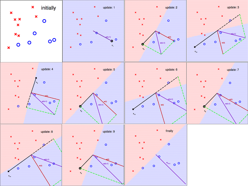
图3 PLA 知"错"就"改"的过程

从图中可以看出 确实在PLA的指导下，慢慢接近心目中的 。

我们知道在数据线性可分的前提下，我们心目中有个完美的 ，它能够完美的把圈圈和叉叉区分开来。那么如何证明PLA能够使 不断接近呢？

这里就要用到夹角余弦的公式，如果 更新之后的 与 之间的夹角余弦变大(夹角变小)了，则我们可以说PLA是有效的。

 

2.2 Linear Regression

 

2.2.1 线性回归模型

线性回归假设特征和结果满足线性关系，属于监督学习的范畴。其估计函数为：

θ在为未知参数，上式采用向量表示为：

机器学习算法是的主要目的是找到最能够对数据做出合理解释的模型，这个模型是假设函数，数学推导基本遵循这样的思路

1. 假设函数
2. 为了找到最好的假设函数，需要找到合理的评估标准，一般来说使用损失函数作为评估标准
3. 根据损失函数推出目标函数
4. 现在问题转换成为如何找到目标函数的最优解，也就是目标函数的最优化

回归分析最初的目的是估计模型参数以便达到对数据的最佳拟合。一般

我们对 函数进行评估的函数称为损失函数（cost function）。下式的 函数即为损失函数：

上式得损失函数是对 的估计值与真实值 差的平方和作为错误估计函数，上式中的1/2是为了在求导时就可抵消。如何调整 以使得 取得最小值有很多方法，其中有最小二乘法和梯度下降法。

 

2.2.2 最小二乘法( least square method)

将训练特征表示为X矩阵，结果表示成y向量，仍然是线性回归模型，误差函数不变。那么θ可以直接由下面公式得出

此方法要求X是列满秩的，而且求矩阵的逆比较慢。

 

2.2.3 梯度下降算法（Gradient Descent）

梯度下降算法用于在迭代过程中逐渐降阶，不断更新特征权重向量，从而得到无限接近或拟合的最优特征权重向量 ；梯度下降算法主要有两种,第一种是批量梯度下降(Batch Gradient Descent)算法，此种方式实现过程是对权重向量进行累加，然后批量更新的一种方式，一般不实用于大规模数据集处理；另外一种是随机梯度下降(Stochastic Gradient Descent)算法，这种方式对给定训练数据集中每个对象都进行权重计算和更新，在某些情况下容易收敛到局部最优解上。

梯度下降原理：将函数比作一座山，我们站在某个山坡上，往四周看，从哪个方向向下走一小步，能够下降的最快。

1. 先确定向下一步的步伐大小，我们称为Learning rate；
2. 任意给定一个初始值；
3. 确定一个向下的方向，并向下走预先规定的步伐，并更新；
4. 当下降的高度小于某个定义的值，则停止下降；

 

 

 

批量梯度下降算法的理论公式：

随机梯度下降算法的理论公式：

批量梯度下降算法每次更新 中的一个元素需要处理整个输入样本集。随机梯度下降法每次更新参数向量时，只按照其中一个参数的梯度方向更新参数。

最小二乘法能够很好的评估线性回归的拟合度，而利用梯度下降法能找到最能满足最小二乘法的权重向量。可以这样理解，最小二乘法是判断线性回归拟合度最好的cost function，而梯度下降是用来找到cost function中对应向量的方法。

 

2.2.4 Spark MLlib实现线性回归

Spark MLlib库中主要使用随机梯度下降算法。

下面的代码包含加载数据，解析为RDD(译者注：RDD为Spark的弹性数据集)；然后利用线性回归和随机梯度下降算法构建一个线性模型，并进行预测，最后计算均方误差(Mean Squared Errors)来对模型进行评估。

Scala code

import org.apache.spark.mllib.regression.LinearRegressionWithSGD

import org.apache.spark.mllib.regression.LabeledPoint

 

// Load and parse the data

val data = sc.textFile("mllib/data/ridge-data/lpsa.data")

val parsedData = data.map { line =>

val parts = line.split(',')

LabeledPoint(parts(0).toDouble, parts(1).split(' ').map(x => x.toDouble).toArray)

}

 

// Building the model

val numIterations = 20

val model = LinearRegressionWithSGD.train(parsedData, numIterations)

 

// Evaluate model on training examples and compute training error

val valuesAndPreds = parsedData.map { point =>

val prediction = model.predict(point.features)

(point.label, prediction)

}

val MSE = valuesAndPreds.map{ case(v, p) => math.pow((v - p), 2)}.reduce(_ + _)/valuesAndPreds.count 

println("training Mean Squared Error = " + MSE) 

 

 

2.3 Classification and Logistic Regression

 

2.3.1 逻辑回归算法原理

一般来说，回归不应用在分类问题上，因为回归是连续型模型，而且受噪声影响比较大。如果非要应用则可以使用逻辑回归。

逻辑回归本质上是线性回归，只是在特征到结果的映射中加入了一层函数映射，即先把特征线性求和，然后使用函数g(z)将最为假设函数来预测。g(z)可以将连续值映射到0和1上。

 

 

 

 

 

 

 

 

 

 

 

可以看到与线性回归类似，只是换成了，而实际上就是经过g(z)映射过来的。

 

2.3.2 Classifying MNIST digits using Logistic Regression

 

Python code  

"""

This tutorial introduces logistic regression using Theano and stochastic

gradient descent.

 

Logistic regression is a probabilistic, linear classifier. It is parametrized

by a weight matrix :math:`W` and a bias vector :math:`b`. Classification is

done by projecting data points onto a set of hyperplanes, the distance to

which is used to determine a class membership probability.

 

Mathematically, this can be written as:

 

.. math::

 P(Y=i|x, W,b) &= softmax_i(W x + b) \\

 &= \frac {e^{W_i x + b_i}} {\sum_j e^{W_j x + b_j}}

 

 

The output of the model or prediction is then done by taking the argmax of

the vector whose i'th element is P(Y=i|x).

 

.. math::

 

 y_{pred} = argmax_i P(Y=i|x,W,b)

 

 

This tutorial presents a stochastic gradient descent optimization method

suitable for large datasets.

 

 

References:

 

 - textbooks: "Pattern Recognition and Machine Learning" -

 Christopher M. Bishop, section 4.3.2

 

"""

__docformat__ = 'restructedtext en'

 

import cPickle

import gzip

import os

import sys

import time

 

import numpy

 

import theano

import theano.tensor as T

 

 

class LogisticRegression(object): 

"""Multi-class Logistic Regression Class

 

 The logistic regression is fully described by a weight matrix :math:`W`

 and bias vector :math:`b`. Classification is done by projecting data

 points onto a set of hyperplanes, the distance to which is used to

 determine a class membership probability.

 """

 

def __init__(self, input, n_in, n_out): 

""" Initialize the parameters of the logistic regression

 

 :type input: theano.tensor.TensorType

 :param input: symbolic variable that describes the input of the

 architecture (one minibatch)

 

 :type n_in: int

 :param n_in: number of input units, the dimension of the space in

 which the datapoints lie

 

 :type n_out: int

 :param n_out: number of output units, the dimension of the space in

 which the labels lie

 

 """

# start-snippet-1

# initialize with 0 the weights W as a matrix of shape (n_in, n_out)

self.W = theano.shared( 

 value=numpy.zeros( 

 (n_in, n_out), 

 dtype=theano.config.floatX 

 ), 

 name='W', 

 borrow=True

 ) 

# initialize the baises b as a vector of n_out 0s

self.b = theano.shared( 

 value=numpy.zeros( 

 (n_out,), 

 dtype=theano.config.floatX 

 ), 

 name='b', 

 borrow=True

 ) 

 

# symbolic expression for computing the matrix of class-membership

# probabilities

# Where:

# W is a matrix where column-k represent the separation hyper plain for

# class-k

# x is a matrix where row-j represents input training sample-j

# b is a vector where element-k represent the free parameter of hyper

# plain-k

self.p_y_given_x = T.nnet.softmax(T.dot(input, self.W) + self.b) 

 

# symbolic description of how to compute prediction as class whose

# probability is maximal

self.y_pred = T.argmax(self.p_y_given_x, axis=1) 

# end-snippet-1

 

# parameters of the model

self.params = [self.W, self.b] 

 

def negative_log_likelihood(self, y): 

"""Return the mean of the negative log-likelihood of the prediction

 of this model under a given target distribution.

 

 .. math::

 

 \frac{1}{|\mathcal{D}|} \mathcal{L} (\theta=\{W,b\}, \mathcal{D}) =

 \frac{1}{|\mathcal{D}|} \sum_{i=0}^{|\mathcal{D}|}

 \log(P(Y=y^{(i)}|x^{(i)}, W,b)) \\

 \ell (\theta=\{W,b\}, \mathcal{D})

 

 :type y: theano.tensor.TensorType

 :param y: corresponds to a vector that gives for each example the

 correct label

 

 Note: we use the mean instead of the sum so that

 the learning rate is less dependent on the batch size

 """

# start-snippet-2

# y.shape[0] is (symbolically) the number of rows in y, i.e.,

# number of examples (call it n) in the minibatch

# T.arange(y.shape[0]) is a symbolic vector which will contain

# [0,1,2,... n-1] T.log(self.p_y_given_x) is a matrix of

# Log-Probabilities (call it LP) with one row per example and

# one column per class LP[T.arange(y.shape[0]),y] is a vector

# v containing [LP[0,y[0]], LP[1,y[1]], LP[2,y[2]], ...,

# LP[n-1,y[n-1]]] and T.mean(LP[T.arange(y.shape[0]),y]) is

# the mean (across minibatch examples) of the elements in v,

# i.e., the mean log-likelihood across the minibatch.

return -T.mean(T.log(self.p_y_given_x)[T.arange(y.shape[0]), y]) 

# end-snippet-2

 

def errors(self, y): 

"""Return a float representing the number of errors in the minibatch

 over the total number of examples of the minibatch ; zero one

 loss over the size of the minibatch

 

 :type y: theano.tensor.TensorType

 :param y: corresponds to a vector that gives for each example the

 correct label

 """

 

# check if y has same dimension of y_pred

if y.ndim != self.y_pred.ndim: 

raise TypeError( 

'y should have the same shape as self.y_pred', 

 ('y', y.type, 'y_pred', self.y_pred.type) 

 ) 

# check if y is of the correct datatype

if y.dtype.startswith('int'): 

# the T.neq operator returns a vector of 0s and 1s, where 1

# represents a mistake in prediction

return T.mean(T.neq(self.y_pred, y)) 

else: 

raise NotImplementedError() 

 

 

def load_data(dataset): 

''' Loads the dataset

 

 :type dataset: string

 :param dataset: the path to the dataset (here MNIST)

 '''

 

#############

# LOAD DATA #

#############

 

# Download the MNIST dataset if it is not present

 data_dir, data_file = os.path.split(dataset) 

if data_dir == "" and not os.path.isfile(dataset): 

# Check if dataset is in the data directory.

 new_path = os.path.join( 

 os.path.split(__file__)[0], 

"..", 

"data", 

 dataset 

 ) 

if os.path.isfile(new_path) or data_file == 'mnist.pkl.gz': 

 dataset = new_path 

 

if (not os.path.isfile(dataset)) and data_file == 'mnist.pkl.gz': 

import urllib

 origin = ( 

'http://www.iro.umontreal.ca/~lisa/deep/data/mnist/mnist.pkl.gz'

 ) 

print 'Downloading data from %s' % origin 

 urllib.urlretrieve(origin, dataset) 

 

print '... loading data'

 

# Load the dataset

 f = gzip.open(dataset, 'rb') 

 train_set, valid_set, test_set = cPickle.load(f) 

 f.close() 

#train_set, valid_set, test_set format: tuple(input, target)

#input is an numpy.ndarray of 2 dimensions (a matrix)

#witch row's correspond to an example. target is a

#numpy.ndarray of 1 dimensions (vector)) that have the same length as

#the number of rows in the input. It should give the target

#target to the example with the same index in the input.

 

def shared_dataset(data_xy, borrow=True): 

""" Function that loads the dataset into shared variables

 

 The reason we store our dataset in shared variables is to allow

 Theano to copy it into the GPU memory (when code is run on GPU).

 Since copying data into the GPU is slow, copying a minibatch everytime

 is needed (the default behaviour if the data is not in a shared

 variable) would lead to a large decrease in performance.

 """

 data_x, data_y = data_xy 

 shared_x = theano.shared(numpy.asarray(data_x, 

 dtype=theano.config.floatX), 

 borrow=borrow) 

 shared_y = theano.shared(numpy.asarray(data_y, 

 dtype=theano.config.floatX), 

 borrow=borrow) 

# When storing data on the GPU it has to be stored as floats

# therefore we will store the labels as ``floatX`` as well

# (``shared_y`` does exactly that). But during our computations

# we need them as ints (we use labels as index, and if they are

# floats it doesn't make sense) therefore instead of returning

# ``shared_y`` we will have to cast it to int. This little hack

# lets ous get around this issue

return shared_x, T.cast(shared_y, 'int32') 

 

 test_set_x, test_set_y = shared_dataset(test_set) 

 valid_set_x, valid_set_y = shared_dataset(valid_set) 

 train_set_x, train_set_y = shared_dataset(train_set) 

 

 rval = [(train_set_x, train_set_y), (valid_set_x, valid_set_y), 

 (test_set_x, test_set_y)] 

return rval 

 

 

def sgd_optimization_mnist(learning_rate=0.13, n_epochs=1000, 

 dataset='mnist.pkl.gz', 

 batch_size=600): 

"""

 Demonstrate stochastic gradient descent optimization of a log-linear

 model

 

 This is demonstrated on MNIST.

 

 :type learning_rate: float

 :param learning_rate: learning rate used (factor for the stochastic

 gradient)

 

 :type n_epochs: int

 :param n_epochs: maximal number of epochs to run the optimizer

 

 :type dataset: string

 :param dataset: the path of the MNIST dataset file from

 http://www.iro.umontreal.ca/~lisa/deep/data/mnist/mnist.pkl.gz

 

 """

 datasets = load_data(dataset) 

 

 train_set_x, train_set_y = datasets[0] 

 valid_set_x, valid_set_y = datasets[1] 

 test_set_x, test_set_y = datasets[2] 

 

# compute number of minibatches for training, validation and testing

 n_train_batches = train_set_x.get_value(borrow=True).shape[0] / batch_size 

 n_valid_batches = valid_set_x.get_value(borrow=True).shape[0] / batch_size 

 n_test_batches = test_set_x.get_value(borrow=True).shape[0] / batch_size 

 

######################

# BUILD ACTUAL MODEL #

######################

print '... building the model'

 

# allocate symbolic variables for the data

 index = T.lscalar() # index to a [mini]batch

 

# generate symbolic variables for input (x and y represent a

# minibatch)

 x = T.matrix('x') # data, presented as rasterized images

 y = T.ivector('y') # labels, presented as 1D vector of [int] labels

 

# construct the logistic regression class

# Each MNIST image has size 28*28

 classifier = LogisticRegression(input=x, n_in=28 * 28, n_out=10) 

 

# the cost we minimize during training is the negative log likelihood of

# the model in symbolic format

 cost = classifier.negative_log_likelihood(y) 

 

# compiling a Theano function that computes the mistakes that are made by

# the model on a minibatch

 test_model = theano.function( 

 inputs=[index], 

 outputs=classifier.errors(y), 

 givens={ 

 x: test_set_x[index * batch_size: (index + 1) * batch_size], 

 y: test_set_y[index * batch_size: (index + 1) * batch_size] 

 } 

 ) 

 

 validate_model = theano.function( 

 inputs=[index], 

 outputs=classifier.errors(y), 

 givens={ 

 x: valid_set_x[index * batch_size: (index + 1) * batch_size], 

 y: valid_set_y[index * batch_size: (index + 1) * batch_size] 

 } 

 ) 

 

# compute the gradient of cost with respect to theta = (W,b)

 g_W = T.grad(cost=cost, wrt=classifier.W) 

 g_b = T.grad(cost=cost, wrt=classifier.b) 

 

# start-snippet-3

# specify how to update the parameters of the model as a list of

# (variable, update expression) pairs.

 updates = [(classifier.W, classifier.W - learning_rate * g_W), 

 (classifier.b, classifier.b - learning_rate * g_b)] 

 

# compiling a Theano function `train_model` that returns the cost, but in

# the same time updates the parameter of the model based on the rules

# defined in `updates`

 train_model = theano.function( 

 inputs=[index], 

 outputs=cost, 

 updates=updates, 

 givens={ 

 x: train_set_x[index * batch_size: (index + 1) * batch_size], 

 y: train_set_y[index * batch_size: (index + 1) * batch_size] 

 } 

 ) 

# end-snippet-3

 

###############

# TRAIN MODEL #

###############

print '... training the model'

# early-stopping parameters

 patience = 5000 # look as this many examples regardless

 patience_increase = 2 # wait this much longer when a new best is

# found

 improvement_threshold = 0.995 # a relative improvement of this much is

# considered significant

 validation_frequency = min(n_train_batches, patience / 2) 

# go through this many

# minibatche before checking the network

# on the validation set; in this case we

# check every epoch

 

 best_validation_loss = numpy.inf 

 test_score = 0.

 start_time = time.clock() 

 

 done_looping = False

 epoch = 0

while (epoch < n_epochs) and (not done_looping): 

epoch = epoch + 1

for minibatch_index in xrange(n_train_batches): 

 

 minibatch_avg_cost = train_model(minibatch_index) 

# iteration number

iter = (epoch - 1) * n_train_batches + minibatch_index 

 

if (iter + 1) % validation_frequency == 0: 

# compute zero-one loss on validation set

 validation_losses = [validate_model(i) 

for i in xrange(n_valid_batches)] 

 this_validation_loss = numpy.mean(validation_losses) 

 

print( 

'epoch %i, minibatch %i/%i, validation error %f %%' %

 ( 

 epoch, 

 minibatch_index + 1, 

 n_train_batches, 

 this_validation_loss * 100.

 ) 

 ) 

 

# if we got the best validation score until now

if this_validation_loss < best_validation_loss: 

#improve patience if loss improvement is good enough

if this_validation_loss < best_validation_loss * \ 

 improvement_threshold: 

 patience = max(patience, iter * patience_increase) 

 

 best_validation_loss = this_validation_loss 

# test it on the test set

 

 test_losses = [test_model(i) 

for i in xrange(n_test_batches)] 

 test_score = numpy.mean(test_losses) 

 

print( 

 ( 

' epoch %i, minibatch %i/%i, test error of'

' best model %f %%'

 ) %

 ( 

 epoch, 

 minibatch_index + 1, 

 n_train_batches, 

 test_score * 100.

 ) 

 ) 

 

if patience <= iter: 

 done_looping = True

break

 

 end_time = time.clock() 

print( 

 ( 

'Optimization complete with best validation score of %f %%,'

'with test performance %f %%'

 ) 

% (best_validation_loss * 100., test_score * 100.) 

) 

print 'The code run for %d epochs, with %f epochs/sec' % ( 

 epoch, 1. * epoch / (end_time - start_time)) 

print >> sys.stderr, ('The code for file ' +

 os.path.split(__file__)[1] +

' ran for %.1fs' % ((end_time - start_time))) 

 

if __name__ == '__main__': 

 sgd_optimization_mnist() 

 

The user can learn to classify MNIST digits with SGD logistic regression, by typing, from within the DeepLearningTutorials folder:

python code/logistic_sgd.py

The output one should expect is of the form :

...

epoch 72, minibatch 83/83, validation error 7.510417 %

epoch 72, minibatch 83/83, test error of best model 7.510417 %

epoch 73, minibatch 83/83, validation error 7.500000 %

epoch 73, minibatch 83/83, test error of best model 7.489583 %

Optimization complete with best validation score of 7.500000 %,with test performance 7.489583 %

The code run for 74 epochs, with 1.936983 epochs/sec

On an Intel(R) Core(TM)2 Duo CPU E8400 @ 3.00 Ghz the code runs with approximately 1.936 epochs/sec and it took 75 epochs to reach a test error of 7.489%. On the GPU the code does almost 10.0 epochs/sec. For this instance we used a batch size of 600.

 

 

2.4 Softmax Regression

 

2.4.1 简介

本节的主要内容是Softmax回归模型，该模型是logistic回归模型在多分类问题上的推广，在多分类问题中，类标签 可以取两个以上的值。Softmax回归模型对于诸如MNIST手写数字分类等问题是很有用的，该问题的目的是辨识10个不同的单个数字。Softmax回归是有监督的，不过后面也会介绍它与深度学习/无监督学习方法的结合（MNIST 是一个手写数字识别库，由NYU 的Yann LeCun 等人维护。http://yann.lecun.com/exdb/mnist/ ）。

回想一下在 logistic 回归中，我们的训练集由 个已标记的样本构成： ，其中输入特征（我们对符号的约定如下：特征向量 的维度为 ，其中 对应截距项 ）。由于 logistic 回归是针对二分类问题的，因此类标记 。假设函数(hypothesis function) 如下：

我们将训练模型参数 ，使其能够最小化代价函数 ：

在 softmax回归中，我们解决的是多分类问题（相对于 logistic 回归解决的二分类问题），类标 可以取 个不同的值（而不是 2 个）。因此，对于训练集 ，我们有 。（注意此处的类别下标从 1 开始，而不是 0）。例如，在 MNIST 数字识别任务中，我们有 个不同的类别。

对于给定的测试输入 ，我们想用假设函数针对每一个类别 j 估算出概率值 。也就是说，我们想估计 的每一种分类结果出现的概率。因此，我们的假设函数将要输出一个 维的向量（向量元素的和为1）来表示这 个估计的概率值。 具体地说，我们的假设函数 形式如下：

 

其中 是模型的参数。请注意 这一项对概率分布进行归一化，使得所有概率之和为 1 。

为了方便起见，我们同样使用符号 来表示全部的模型参数。在实现Softmax回归时，将 用一个 的矩阵来表示会很方便，该矩阵是将 按行罗列起来得到的，如下所示：

 

2.4.2 cost function

现在我们来介绍 softmax 回归算法的代价函数。在下面的公式中， 是示性函数，其取值规则为：

值为真的表达式 ； 值为假的表达式

举例来说，表达式 的值为1 ，的值为0。

Cost function 为：

值得注意的是，上述公式是logistic回归代价函数的推广。logistic回归的 cost function可以改为：

可以看到，Softmax代价函数与logistic 代价函数在形式上非常类似，只是在Softmax损失函数中对类标记的 个可能值进行了累加。注意在Softmax回归中将 分类为类别 的概率为：

.

对于 的最小化问题，我们使用迭代的优化算法（例如梯度下降法，或 L-BFGS）。经过求导，我们得到梯度公式如下：

让我们来回顾一下符号 "" 的含义。 本身是一个向量，它的第 个元素 是 对 的第 个分量的偏导数。

有了上面的偏导数公式以后，我们就可以将它代入到梯度下降法等算法中，来最小化 。 例如，在梯度下降法的标准实现中，每一次迭代需要进行如下更新: () 。

实现 softmax 回归算法时，我们通常会使用上述cost function 的一个改进版本，具体来说就是和权重衰减(weight decay)一起使用。

 

2.4.3 Softmax回归模型参数化的特点

Softmax 回归有一个不寻常的特点：它有一个"冗余"的参数集。为了便于阐述这一特点，假设我们从参数向量 中减去了向量 ，这时，每一个 都变成了 ()。此时假设函数变成了以下的式子：

换句话说，从 中减去 完全不影响假设函数的预测结果！这表明前面的 softmax 回归模型中存在冗余的参数。更正式一点来说， Softmax 模型被过度参数化了。对于任意一个用于拟合数据的假设函数，可以求出多组参数值，这些参数得到的是完全相同的假设函数 。
进一步而言，如果参数 是代价函数 的极小值点，那么 同样也是它的极小值点，其中 可以为任意向量。因此使 最小化的解不是唯一的。（有趣的是，由于 仍然是一个凸函数，因此梯度下降时不会遇到局部最优解的问题。但是 Hessian 矩阵是奇异的不可逆的，这会直接导致采用牛顿法优化就遇到数值计算的问题）

注意，当 时，我们总是可以将 替换为 （即替换为全零向量），并且这种变换不会影响假设函数。因此我们可以去掉参数向量 （或者其他 中的任意一个）而不影响假设函数的表达能力。实际上，与其优化全部的 个参数 （其中 ），我们可以令 ，只优化剩余的 个参数，这样算法依然能够正常工作。
在实际应用中，为了使算法实现更简单清楚，往往保留所有参数 ，而不任意地将某一参数设置为 0。但此时我们需要对代价函数做一个改动：加入权重衰减。权重衰减可以解决 softmax 回归的参数冗余所带来的数值问题。

 

2.4.4 权重衰减

我们通过添加一个权重衰减项 来修改代价函数，这个衰减项会惩罚过大的参数值，现在我们的代价函数变为：

有了权重衰减项后 ( )，代价函数就变成了严格的凸函数，这样就可以保证得到唯一的解了。此时的 Hessian矩阵变为可逆矩阵，并且因为 是凸函数，梯度下降法和 L-BFGS 等算法可以保证收敛到全局最优解。

为了使用优化算法，我们需要求得这个新函数 的导数，如下：

通过最小化 ，我们就能实现一个可用的 softmax 回归模型。

 

2.4.5 Softmax回归与Logistic 回归的关系

当类别数 时，softmax 回归退化为 logistic 回归。这表明 softmax 回归是 logistic 回归的一般形式。具体地说，当 时，softmax 回归的假设函数为：

利用softmax回归参数冗余的特点，我们令 ，并且从两个参数向量中都减去向量 ，得到:

因此，用 来表示，我们就会发现 softmax 回归器预测其中一个类别的概率为 ，另一个类别概率的为 ，这与 logistic回归是一致的。

 

2.4.6 Softmax 回归 vs. k 个二元分类器

如果你在开发一个音乐分类的应用，需要对k种类型的音乐进行识别，那么是选择使用 softmax 分类器呢，还是使用 logistic 回归算法建立 k 个独立的二元分类器呢？

这一选择取决于你的类别之间是否互斥，互斥的情况下选择 softmax 回归，否则选用 k 个二分类的逻辑回归分类器。例如，如果你有四个类别的音乐，分别为：古典音乐、乡村音乐、摇滚乐和爵士乐，那么你可以假设每个训练样本只会被打上一个标签（即：一首歌只能属于这四种音乐类型的其中一种），此时你应该使用类别数 k = 4 的softmax回归。（如果在你的数据集中，有的歌曲不属于以上四类的其中任何一类，那么你可以添加一个"其他类"，并将类别数 k 设为5。）

如果你的四个类别如下：人声音乐、舞曲、影视原声、流行歌曲，那么这些类别之间并不是互斥的。例如：一首歌曲可以来源于影视原声，同时也包含人声 。这种情况下，使用4个二分类的 logistic 回归分类器更为合适。这样，对于每个新的音乐作品 ，我们的算法可以分别判断它是否属于各个类别。

 

2.5 Generative Learning algorithms

 

2.5.1 Gaussian discriminant analysis ( GDA )

1) 多值正态分布

 

多变量正态分布描述的是n维随机变量的分布情况，这里的变成了向量，也变成了矩阵。写作。假设有n个随机变量,。的第i个分量是，而。

概率密度函数如下：

其中 是 的行列式， 是协方差矩阵，而且是对称半正定的。

 

Here're some examples of what the density of a Gaussian distribution look like:

The left-most figure shows a Gaussian with mean zero (that is, the 2x1 zero-vector) and covariance matrix Σ = I (the 2x2 identity matrix). A Gaussian with zero mean and identity covariance is also called the standard normal distribution. The middle figure shows the density of a Gaussian with zero mean and Σ = 0.6I; and in the rightmost figure shows one with , Σ = 2I. We see that as Σ becomes larger, the Gaussian becomes more "spread-out," and as it becomes smaller, the distribution becomes more "compressed." Lets look at some more examples.

The figures above show Gaussians with mean 0, and with covariance

matrices respectively

.

The leftmost figure shows the familiar standard normal distribution, and we see that as we increase the off-diagonal entry in Σ, the density becomes more "compressed" towards the 45^◦line (given by x₁ = x₂). We can see this more clearly when we look at the contours of the same three densities:

Here's one last set of examples generated by varying Σ:

The plots above used, respectively,

.

From the leftmost and middle figures, we see that by decreasing the diagonal elements of the covariance matrix, the density now becomes "compressed" again, but in the opposite direction. Lastly, as we vary the parameters, more generally the contours will form ellipses (the rightmost figure showing an example).

As our last set of examples, fixing Σ = I, by varying µ, we can also move the mean of the density around.

The figures above were generated using Σ = I, and respectively

.

 

2) Gaussian Discriminant Analysis model

如果输入特征x是连续型随机变量，那么可以使用高斯判别分析模型来确定p(x|y)。

模型如下：

y	∼	Bernoulli(φ)
x|y = 0	∼	N(µ0,Σ)
x|y = 1	∼	N(µ1,Σ)

 

输出结果服从伯努利分布，在给定模型下特征符合多值高斯分布。

概率分布函数如下所示：

 

The log-likelihood of the data is given by

.

注意这里的参数有两个，表示在不同的结果模型下，特征均值不同，但我们假设协方差相同。反映在图上就是不同模型中心位置不同，但形状相同。这样就可以用直线来进行分隔判别。

求导后，得到参数估计公式：

 

 

如前面所述，在图上表示为：

直线两边的y 值不同，但协方差矩阵相同，因此形状相同。 不同，因此位置不同。

 

3) GDA and logistic regression

将GDA用条件概率方式来表述的话，如下：

y是x的函数，其中都是参数。

进一步推导出

这里的是的函数。

这个形式就是logistic回归的形式。

也就是说如果p(x|y)符合多元高斯分布，那么p(y|x)符合logistic回归模型。反之，不成立。为什么反过来不成立呢？因为GDA有着更强的假设条件和约束。

如果认定训练数据满足多元高斯分布，那么GDA能够在训练集上是最好的模型。然而，我们往往事先不知道训练数据满足什么样的分布，不能做很强的假设。Logistic回归的条件假设要弱于GDA，因此更多的时候采用logistic回归的方法。

例如，训练数据满足泊松分布，

，那么p(y|x)也是logistic回归的。这个时候如果采用GDA，那么效果会比较差，因为训练数据特征的分布不是多元高斯分布，而是泊松分布。这也是logistic回归用的更多的原因。

 

2.5.2 朴素贝叶斯 ( Naive Bayes )

1) 概述

贝叶斯分类的基础是概率推理，就是在各种条件的存在不确定，仅知其出现概率的情况下，如何完成推理和决策任务。概率推理是与确定性推理相对应的。而朴素贝叶斯分类器是基于独立假设的，即假设样本每个特征与其他特征都不相关。

朴素贝叶斯分类器依靠精确的自然概率模型，在有监督学习的样本集中能获取得非常好的分类效果。在许多实际应用中，朴素贝叶斯模型参数估计使用最大似然估计方法，换而言之朴素贝叶斯模型能工作并没有用到贝叶斯概率或者任何贝叶斯模型。

尽管是带着这些朴素思想和过于简单化的假设，但朴素贝叶斯分类器在很多复杂的现实情形中仍能够取得相当好的效果。2004年，一篇分析贝叶斯分类器问题的文章揭示了朴素贝叶斯分类器取得看上去不可思议的分类效果的若干理论上的原因。尽管如此，2006年有一篇文章详细比较了各种分类方法，发现更新的方法（如boosted trees和随机森林）的性能超过了贝叶斯分类器。朴素贝叶斯分类器的一个优势在于只需要根据少量的训练数据估计出必要的参数（变量的均值和方差）。由于变量独立假设，只需要估计各个变量的方法，而不需要确定整个协方差矩阵。

 

2) 朴素贝叶斯概率模型

理论上，概率模型分类器是一个条件概率模型。

独立的类别变量有若干类别，条件依赖于若干特征变量 ,,...,。但问题在于如果特征数量较大或者每个特征能取大量值时，基于概率模型列出概率表变得不现实。所以我们修改这个模型使之变得可行。 贝叶斯定理有以下式子：

用朴素的语言可以表达为：

实际中，我们只关心分式中的分子部分，因为分母不依赖于而且特征的值是给定的，于是分母可以认为是一个常数。这样分子就等价于联合分布模型。

重复使用链式法则，可将该式写成条件概率的形式，如下所示：

现在"朴素"的条件独立假设开始发挥作用:假设每个特征对于其他特征,是条件独立的。这就意味着

对于，所以联合分布模型可以表达为

这意味着上述假设下，类变量的条件分布可以表达为：

其中(证据因子)是一个只依赖与等的缩放因子，当特征变量的值已知时是一个常数。 由于分解成所谓的类先验概率和独立概率分布，上述概率模型的可掌控性得到很大的提高。如果这是一个分类问题，且每个可以表达为个参数，于是相应的朴素贝叶斯模型有(k − 1) + n r k个参数。实际应用中，通常取（二分类问题）， (伯努利分布作为特征），因此模型的参数个数为，其中是二值分类特征的个数。

 

3) Naive Bayes in Spark MLlib

MLlib supports multinomial naive Bayes, which is typically used for document classification. Within that context, each observation is a document and each feature represents a term whose value is the frequency of the term. Feature values must be nonnegative to represent term frequencies. Additive smoothing ( also called Laplace smoothing ) can be used by setting the parameter λ  (default to 1.0  ). For document classification, the input feature vectors are usually sparse, and sparse vectors should be supplied as input to take advantage of sparsity. Since the training data is only used once, it is not necessary to cache it.

NaiveBayes implements multinomial naive Bayes. It takes an RDD of LabeledPoint and an optional smoothing parameter lambda as input, and output a NaiveBayesModel, which can be used for evaluation and prediction.

Scala code

 

import org.apache.spark.mllib.classification.NaiveBayes

import org.apache.spark.mllib.linalg.Vectors

import org.apache.spark.mllib.regression.LabeledPoint

 

val data = sc.textFile("data/mllib/sample_naive_bayes_data.txt")

val parsedData = data.map { line =>

val parts = line.split(',')

LabeledPoint(parts(0).toDouble, Vectors.dense(parts(1).split(' ').map(_.toDouble)))

}

// Split data into training (60%) and test (40%).

val splits = parsedData.randomSplit(Array(0.6, 0.4), seed = 11L)

val training = splits(0)

val test = splits(1)

 

val model = NaiveBayes.train(training, lambda = 1.0)

 

val predictionAndLabel = test.map(p => (model.predict(p.features), p.label))

val accuracy = 1.0 * predictionAndLabel.filter(x => x._1 == x._2).count() / test.count()

  

2.5.3 Laplace smoothing

 

In statistics, additive smoothing, also called Laplace smoothing (not to be confused with Laplacian smoothing), or Lidstone smoothing, is a technique used to smooth categorical data. Given an observation x = (x₁, …, x_d) from a multinomial distribution with N trials and parameter vector θ = (θ₁, …, θ_d), a "smoothed" version of the data gives the estimator:

 

 

2.6 Support Vector Machines

 

2.6.1 Introduction

与复杂的公式推导相对应的是支持向量机（Support Vector Machines -- SVM）清晰明了的算法思想。SVM不像逻辑回归去拟合样本点，而是在样本中去选着最优的分隔线，而为了判别哪条分隔线更好，引入了几何间隔最大化的目标。SVM的目标是寻找一个超平面，使得离超平面比较近的点能有更大的间距。也就是我们不考虑所有的点都必须远离超平面，我们关心求得的超平面能够让所有的点中离它最近的点（支持向量）的间距最大。

本节后面的推导都是解决目标函数最优化，在解决最优化过程中的w可由特征向量内积表示（w的具体含义在后面介绍），进而引入核函数。在优化求解的复杂问题，被拉格朗日对偶和SMO算法化解，将SVM推向极致。

 

2.6.2 由逻辑回归引出SVM

Logistic回归目的是从特征学习出一个0/1分类模型，而这个模型是将特性的线性组合作为自变量，由于自变量的取值范围是负无穷到正无穷。因此，使用logistic函数（或称作sigmoid函数）将自变量映射到(0,1)上，映射后的值被认为是属于y=1的概率。

形式化表示就是：

 

当我们要判别一个新来的特征属于哪个类时，只需求，若大于0.5就是y=1的类，反之属于y=0类。

再审视一下，发现只和有关，>0，那么，g(z)只不过是用来映射，真实的类别决定权还在。还有当时，=1，反之=0。如果我们只从出发，希望模型达到的目标无非就是让训练数据中y=1的特征，而是y=0的特征。Logistic回归就是要学习得到，使得正例的特征远大于0，负例的特征远小于0，强调在全部训练实例上达到这个目标。

图形化表示如下：

 

 

我们这次使用的结果标签是y=-1,y=1，替换在logistic回归中使用的y=0和y=1。同时将替换成w和b。以前的，其中认为。现在我们替换为b，后面替换为（即）。这样，我们让，进一步。也就是说除了y由y=0变为y=-1，只是标记不同外，与logistic回归的形式化表示没区别。再明确下假设函数

 

 

上一节提到过我们只需考虑的正负问题，而不用关心g(z)，因此我们这里将g(z)做一个简化，将其简单映射到y=-1和y=1上。映射关系如下：

 

 

2.6.3 function and geometric margin

给定一个训练样本，x是特征，y是结果标签。i表示第i个样本。我们定义函数间隔如下：

可想而知，当时，在我们的g(z)定义中，，的值实际上就是。反之亦然。为了使函数间隔最大（更大的信心确定该例是正例还是反例），当时，应该是个大正数，反之是个大负数。因此函数间隔代表了我们认为特征是正例还是反例的确信度。

继续考虑w和b，如果同时加大w和b，比如在前面乘个系数比如2，那么所有点的函数间隔都会增大二倍，这个对求解问题来说不应该有影响，因为我们要求解的是，同时扩大w和b对结果是无影响的。这样，我们为了限制w和b，可能需要加入归一化条件，毕竟求解的目标是确定唯一一个w和b，而不是多组线性相关的向量。这个归一化一会再考虑。

上面我们定义的函数间隔是针对某一个样本的，现在我们定义全局样本上的函数间隔

说白了就是在训练样本上分类正例和负例确信度最小那个函数间隔。

接下来定义几何间隔：

 

 

假设我们有了B点所在的分割面。任何其他一点，比如A到该面的距离以表示，假设B就是A在分割面上的投影。我们知道向量BA的方向是（分割面的梯度），单位向量是。A点是，所以B点是x=（利用初中的几何知识），带入得，

 

当时，不就是函数间隔吗？是的，前面提到的函数间隔归一化结果就是几何间隔。他们为什么会一样呢？因为函数间隔是我们定义的，在定义的时候就有几何间隔的色彩。同样，同时扩大w和b，w扩大几倍，就扩大几倍，结果无影响。同样定义全局的几何间隔：

 

 

2.6.4 optimal margin classifier

 

前面提到SVM的目标是寻找一个超平面，使得离超平面比较近的点能有更大的间距。形象的说，我们将上面的图看作是一张纸，我们要找一条折线，按照这条折线折叠后，离折线最近的点的间距比其他折线都要大。

 

 

 

2.6.5 拉格朗日对偶（Lagrange duality）

存在等式约束的极值求法：

 

不等式约束的极值求法：

 

 

 

 

2.6.6 optimal margin classifier revisited

 

重新回到SVM的优化问题：

 

 

从KKT条件得知只有函数间隔是1（离超平面最近的点）的线性约束式前面的系数，也就是说这些约束式，对于其他的不在线上的点()，极值不会在他们所在的范围内取得，因此前面的系数.注意每一个约束即是一个训练样本。

 

 

实线是最大间隔超平面，假设×号的是正例，圆圈的是负例。在虚线上的点就是函数间隔是1的点，那么他们前面的系数，其他点都是。这三个点称作支持向量。

构造拉格朗日函数

这里我们将向量内积表示为

此时的拉格朗日函数只包含了变量。然而我们求出了才能得到w和b。

接着是极大化的过程，

前面提到过对偶问题和原问题满足的几个条件，首先由于目标函数和线性约束都是凸函数，而且这里不存在等式约束h。存在w使得对于所有的i，。因此，一定存在使得是原问题的解，是对偶问题的解。在这里，求就是求了。

如果求出了，根据即可求出w（也是，原问题的解）。然后

即可求出b。即离超平面最近的正的函数间隔要等于离超平面最近的负的函数间隔。

 

2.6.7 Kernels

待补充。

 

2.6.8 Spark MLlib -- SVM with SGD

 

Regularizers in Spark MLlib

The purpose of the regularizer is to encourage simple models and avoid overfitting. We support the following regularizers in MLlib:

 

 

Here sign(w)is the vector consisting of the signs (±1) of all the entries of w.

L2-regularized problems are generally easier to solve than L1-regularized due to smoothness. However, L1 regularization can help promote sparsity in weights leading to smaller and more interpretable models, the latter of which can be useful for feature selection. It is not recommended to train models without any regularization, especially when the number of training examples is small.

 

下面的代码片段演示如何加载示例数据集、 执行训练算法，并计算模型预测结果的训练误差。

Scala code  

import org.apache.spark.SparkContext

import org.apache.spark.mllib.classification.SVMWithSGD

import org.apache.spark.mllib.evaluation.BinaryClassificationMetrics

import org.apache.spark.mllib.regression.LabeledPoint

import org.apache.spark.mllib.linalg.Vectors

import org.apache.spark.mllib.util.MLUtils

 

// Load training data in LIBSVM format.

val data = MLUtils.loadLibSVMFile(sc, "data/mllib/sample_libsvm_data.txt")

 

// Split data into training (60%) and test (40%).

val splits = data.randomSplit(Array(0.6, 0.4), seed = 11L)

val training = splits(0).cache()

val test = splits(1)

 

// Run training algorithm to build the model

val numIterations = 100

val model = SVMWithSGD.train(training, numIterations)

 

// Clear the default threshold.

model.clearThreshold()

 

// Compute raw scores on the test set. 

val scoreAndLabels = test.map { point =>

val score = model.predict(point.features)

(score, point.label)

}

 

// Get evaluation metrics.

val metrics = new BinaryClassificationMetrics(scoreAndLabels)

val auROC = metrics.areaUnderROC()

 

println("Area under ROC = " + auROC)

 

默认情况下的 SVMWithSGD.train() 方法执行 L2 正则化且正则化参数设置为 1.0。如果我们想要修改算法的运算参数，可以创建 SVMWithSGD 新对象并调用参数优化的 setter 方法。例如，下面的代码产生 L1 正则化的变形的支持向量机与正则化参数设置为 0.1，并运行 200 次迭代训练算法。

 

Scala code

import org.apache.spark.mllib.optimization.L1Updater

 

val svmAlg = new SVMWithSGD()

svmAlg.optimizer.

 setNumIterations(200).

 setRegParam(0.1).

 setUpdater(new L1Updater)

val modelL1 = svmAlg.run(training)

 

 

 

2.7 神经网络

 

2.7.1 概述

以监督学习为例，假设我们有训练样本集 ，那么神经网络算法能够提供一种复杂且非线性的假设模型 ，它具有参数 ，可以以此参数来拟合我们的数据。
为了描述神经网络，我们先从最简单的神经网络讲起，这个神经网络仅由一个"神经元"构成，以下即是这个"神经元"的图示：

这个"神经元"是一个以 及截距 为输入值的运算单元，其输出为 ，其中函数 被称为"激活函数"。在此选用sigmoid函数作为激活函数

可以看出，这个单一"神经元"的输入－输出映射关系其实就是一个逻辑回归（logistic regression）。

除了sigmoid函数以外，也可以选择双曲正切函数（tanh）：

 

以下分别是sigmoid及tanh的函数图像

函数是sigmoid函数的一种变体，它的取值范围为 ，而不是sigmoid函数的 。
注意，与其它地方（包括OpenClassroom公开课以及斯坦福大学CS229课程）不同的是，这里不再令 。取而代之，我们用单独的参数 来表示截距。
最后要说明的是，有一个等式我们以后会经常用到：如果选择 ，也就是sigmoid函数，那么它的导数就是 （如果选择tanh函数，那它的导数就是 ，你可以根据sigmoid（或tanh）函数的定义自行推导这个等式。

 

2.7.2 神经网络模型

所谓神经网络就是将许多个单一"神经元"联结在一起，这样，一个"神经元"的输出就可以是另一个"神经元"的输入。例如，下图就是一个简单的神经网络：

我们使用圆圈来表示神经网络的输入，标上""的圆圈被称为偏置节点，也就是截距项。神经网络最左边的一层叫做输入层，最右的一层叫做输出层（上图中，输出层只有一个节点）。中间所有节点组成的一层叫做隐藏层，因为我们不能在训练样本集中观测到它们的值。同时可以看到，以上神经网络的例子中有3个输入单元（偏置单元不计在内），3个隐藏单元及一个输出单元。
我们用 来表示网络的层数，本例中 ，我们将第 层记为 ，于是 是输入层，输出层是 。本例神经网络有参数 ，其中 （下面的式子中用到）是第 层第 单元与第 层第 单元之间的联接参数（其实就是连接线上的权重，注意标号顺序）， 是第 层第 单元的偏置项。因此在本例中， ， 。注意，没有其他单元连向偏置单元（即偏置单元没有输入），因为它们总是输出 。同时，我们用 表示第 层的节点数（偏置单元不计在内）。
我们用 表示第 层第 单元的激活值（输出值）。当 时， ，也就是第 个输入值（输入值的第 个特征）。对于给定参数集合 ，我们的神经网络就可以按照函数 来计算输出结果。本例神经网络的计算步骤如下：

 

我们用 表示第 层第 单元输入加权和（包括偏置单元），比如， ，则 。

这样我们就可以得到一种更简洁的表示法。这里我们将激活函数 扩展为用向量（分量的形式）来表示，即 ，那么，上面的等式可以更简洁地表示为：

 

我们将上面的计算步骤叫作前向传播。回想一下，之前我们用 表示输入层的激活值，那么给定第 层的激活值 后，第 层的激活值 就可以按照下面步骤计算得到：

 

将参数矩阵化，使用矩阵－向量运算方式，我们就可以利用线性代数的优势对神经网络进行快速求解。
目前为止，我们讨论了一种神经网络，我们也可以构建另一种结构的神经网络（这里结构指的是神经元之间的联接模式），也就是包含多个隐藏层的神经网络。最常见的一个例子是 层的神经网络，第 层是输入层，第 层是输出层，中间的每个层 与层 紧密相联。这种模式下，要计算神经网络的输出结果，我们可以按照之前描述的等式，按部就班，进行前向传播，逐一计算第 层的所有激活值，然后是第 层的激活值，以此类推，直到第 层。这是一个前馈神经网络的例子，因为这种联接图没有闭环或回路。
神经网络也可以有多个输出单元。比如，下面的神经网络有两层隐藏层： 及 ，输出层 有两个输出单元。

 

要求解这样的神经网络，需要样本集 ，其中 。如果你想预测的输出是多个的，那这种神经网络很适用。（比如，在医疗诊断应用中，患者的体征指标就可以作为向量的输入值，而不同的输出值 可以表示不同的疾病存在与否。）

 

 

参考文献

 

[1] Machine Learning Open Class by Andrew Ng in Stanford http://openclassroom.stanford.edu/MainFolder/CoursePage.php?course=MachineLearning

[2] Yu Zheng, Licia Capra, Ouri Wolfson, Hai Yang. Urban Computing: concepts, methodologies, and applications. ACM Transaction on Intelligent Systems and Technology. 5(3), 2014

[3] Jerry Lead http://www.cnblogs.com/jerrylead/

[4]《大数据-互联网大规模数据挖掘与分布式处理》 Anand Rajaraman，Jeffrey David Ullman著，王斌译

[5] UFLDL Tutorial http://deeplearning.stanford.edu/wiki/index.php/UFLDL_Tutorial

[6] Spark MLlib之朴素贝叶斯分类算法 http://selfup.cn/683.html

[7] MLlib - Dimensionality Reduction http://spark.apache.org/docs/latest/mllib-dimensionality-reduction.html

[8] 机器学习中的数学(5)-强大的矩阵奇异值分解(SVD)及其应用 http://www.cnblogs.com/LeftNotEasy/archive/2011/01/19/svd-and-applications.html

[9] 浅谈 mllib 中线性回归的算法实现 http://www.cnblogs.com/hseagle/p/3664933.html

[10] 最大似然估计 http://zh.wikipedia.org/zh-cn/%E6%9C%80%E5%A4%A7%E4%BC%BC%E7%84%B6%E4%BC%B0%E8%AE%A1

[11] Deep Learning Tutorial http://deeplearning.net/tutorial/