Caffe 使用记录（一）mnist手写数字识别

1. 运行它

1. 安装caffe请参考 http://www.cnblogs.com/xuanyuyt/p/5726926.html

　 此例子在官网 http://caffe.berkeleyvision.org/gathered/examples/mnist.html

2. 下载训练和测试数据。caffe识别leveldb或者lmdb格式的数据。

1)这里提供转换好的LEVELDB格式数据集，解压缩到mnist例子目录下

链接：http://pan.baidu.com/s/1gfjXteV 密码：45j6

2)如果要按照官网来转成LMDB格式，那么需要能在windows下运行.sh的程序, 需要安装 Git 和 wgetwin (将wget.exe放入C:\Windows\System32)

运行 D:\caffe-master\data\mnist\get_mnist.sh 这里我们加了一个暂停... read -n1 var

#!/usr/bin/env sh# This scripts downloads the mnist data and unzips it.

DIR="$( cd "$(dirname "$0")" ; pwd -P )"
cd "$DIR"

echo "Downloading..."

for fname in train-images-idx3-ubyte train-labels-idx1-ubyte t10k-images-idx3-ubyte t10k-labels-idx1-ubyte
do
    if [ ! -e $fname ]; then
        wget  http://yann.lecun.com/exdb/mnist/${fname}.gz
        gunzip ${fname}.gz
    fi
done
read -n1 var

运行后我们得到这4个数据文件，分别是测试集图片、测试集标签、训练集图片和训练集标签，图片中文件按行组织：

下载到的原始数据集为二进制文件，需要转换为leveldb或lmdb格式才能被caffe识别

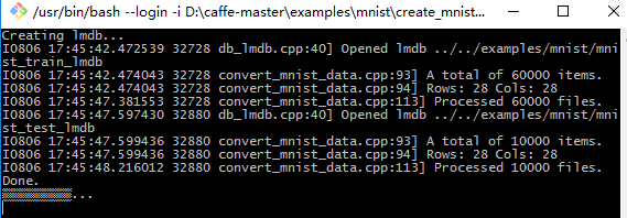
再去运行D:\caffe-master\examples\mnist\create_mnist.sh, 这里路径有点小改动。。。

#!/usr/bin/env sh
        
# This script converts the mnist data into lmdb/leveldb format,
# depending on the value assigned to $BACKEND.
set -e

EXAMPLE=.
DATA=../../data/mnist
BUILD=../../Build/x64/Release

BACKEND="lmdb"

echo "Creating ${BACKEND}..."

rm -rf $EXAMPLE/mnist_train_${BACKEND}
rm -rf $EXAMPLE/mnist_test_${BACKEND}

$BUILD/convert_mnist_data.exe $DATA/train-images-idx3-ubyte \
  $DATA/train-labels-idx1-ubyte $EXAMPLE/mnist_train_${BACKEND} --backend=${BACKEND}
$BUILD/convert_mnist_data.exe $DATA/t10k-images-idx3-ubyte \
  $DATA/t10k-labels-idx1-ubyte $EXAMPLE/mnist_test_${BACKEND} --backend=${BACKEND}

echo "Done."

read -p "回车继续..."

运行后得到mnist_test_lmdb和mnist_train_lmdb两个文件夹

当然你也可以写.bat文件，如下

rd /s /q mnist_train_lmdb 
rd /s /q mnist_test_lmdb

../../Build/x64/Release/convert_mnist_data.exe ../../data/mnist/train-images-idx3-ubyte ../../data/mnist/train-labels-idx1-ubyte mnist_train_lmdb --backend=lmdb 

../../Build/x64/Release/convert_mnist_data.exe ../../data/mnist/t10k-images-idx3-ubyte ../../data/mnist/t10k-labels-idx1-ubyte mnist_test_lmdb --backend=lmdb 
pause

3. 打开lenet_solver.prototxt，这里可以自己试着改几个参数看看最终效果

# The train/test net protocol buffer definition
net: "lenet_train_test.prototxt"
# test_iter specifies how many forward passes the test should carry out.
# In the case of MNIST, we have test batch size 100 and 100 test iterations,
# covering the full 10,000 testing images.
test_iter: 100
# Carry out testing every 500 training iterations.
test_interval: 500
# The base learning rate, momentum and the weight decay of the network.
base_lr: 0.01
momentum: 0.9
weight_decay: 0.0005
# The learning rate policy
lr_policy: "inv"
gamma: 0.0001
power: 0.75
# Display every 100 iterations
display: 100
# The maximum number of iterations
max_iter: 10000
# snapshot intermediate results
snapshot: 5000
snapshot_prefix: "lenet"
# solver mode: CPU or GPU
solver_mode: GPU

4. 打开lenet_train_test.prototxt，注意这里的LMBD和LEVELDB在上面准备数据时你选择的是哪一种，如下

name: "LeNet"
layer {
  name: "mnist"
  type: "Data"
  top: "data"
  top: "label"
  include {
    phase: TRAIN
  }
  transform_param {
    scale: 0.00390625
  }
  data_param {
    source: "mnist_train_lmdb"
    batch_size: 64
    backend: LMDB
  }
}
layer {
  name: "mnist"
  type: "Data"
  top: "data"
  top: "label"
  include {
    phase: TEST
  }
  transform_param {
    scale: 0.00390625
  }
  data_param {
    source: "mnist_test_lmdb"
    batch_size: 100
    backend: LMDB
  }
}
layer {
  name: "conv1"
  type: "Convolution"
  bottom: "data"
  top: "conv1"
  param {
    lr_mult: 1
  }
  param {
    lr_mult: 2
  }
  convolution_param {
    num_output: 20
    kernel_size: 5
    stride: 1
    weight_filler {
      type: "xavier"
    }
    bias_filler {
      type: "constant"
    }
  }
}
layer {
  name: "pool1"
  type: "Pooling"
  bottom: "conv1"
  top: "pool1"
  pooling_param {
    pool: MAX
    kernel_size: 2
    stride: 2
  }
}
layer {
  name: "conv2"
  type: "Convolution"
  bottom: "pool1"
  top: "conv2"
  param {
    lr_mult: 1
  }
  param {
    lr_mult: 2
  }
  convolution_param {
    num_output: 50
    kernel_size: 5
    stride: 1
    weight_filler {
      type: "xavier"
    }
    bias_filler {
      type: "constant"
    }
  }
}
layer {
  name: "pool2"
  type: "Pooling"
  bottom: "conv2"
  top: "pool2"
  pooling_param {
    pool: MAX
    kernel_size: 2
    stride: 2
  }
}
layer {
  name: "ip1"
  type: "InnerProduct"
  bottom: "pool2"
  top: "ip1"
  param {
    lr_mult: 1
  }
  param {
    lr_mult: 2
  }
  inner_product_param {
    num_output: 500
    weight_filler {
      type: "xavier"
    }
    bias_filler {
      type: "constant"
    }
  }
}
layer {
  name: "relu1"
  type: "ReLU"
  bottom: "ip1"
  top: "ip1"
}
layer {
  name: "ip2"
  type: "InnerProduct"
  bottom: "ip1"
  top: "ip2"
  param {
    lr_mult: 1
  }
  param {
    lr_mult: 2
  }
  inner_product_param {
    num_output: 10
    weight_filler {
      type: "xavier"
    }
    bias_filler {
      type: "constant"
    }
  }
}
layer {
  name: "accuracy"
  type: "Accuracy"
  bottom: "ip2"
  bottom: "label"
  top: "accuracy"
  include {
    phase: TEST
  }
}
layer {
  name: "loss"
  type: "SoftmaxWithLoss"
  bottom: "ip2"
  bottom: "label"
  top: "loss"
}

5.新建一个train_lenet.txt文档，添加下面一段，然后改后缀名为.bat

..\..\Build\x64\Release\caffe.exe train --solver="lenet_solver.prototxt" --gpu 0
pause

或者修改train_lenet.sh

#!/usr/bin/env sh
set -e
BUILD=../../Build/x64/Release/
echo "Training lenet_solver.prototxt..."

$BUILD/caffe.exe train --solver=lenet_solver.prototxt $@
echo "Done."

read -p "回车继续..."

6. 然后运行这个bat文件

7. 训练好的模型保存在 lenet_iter_10000.caffemodel， 训练状态保存在lenet_iter_10000.solverstate里

如果要单独测试，新建.txt文件，然后保存为.bat格式，内容如下

../../Build/x64/Release/caffe.exe test -model lenet_train_test.prototxt -weights=lenet_iter_10000.caffemodel -iterations 100
pause 

2. 详细说明

LeNet: the MNIST Classification Model

LeNet network对数字识别效果很出色, 具体请参考论文. 这里与原始的LeNet配置有轻微的差距, 使用了 Rectified Linear Unit (ReLU) activations for the neurons 代替了 the sigmoid activations.

LeNet 结构设计包含了CNN的本质, 这种结构在一些大的模型里如 ImageNet 仍被使用. 总的来说, 它包含一个 convolutional layer 随后是一个 pooling layer, 接着又是一个 convolution layer 和一个 pooling layer, 之后跟着两个 fully connected layers similar to the conventional multilayer perceptrons. 这些在下面这个文件里具体定义了: 

$CAFFE_ROOT/examples/mnist/lenet_train_test.prototxt

Define the MNIST Network

This section explains the lenet_train_test.prototxt model definition that specifies the LeNet model for MNIST handwritten digit classification. We assume that you are familiar with Google Protobuf, and assume that you have read the protobuf definitions used by Caffe, which can be found at $CAFFE_ROOT/src/caffe/proto/caffe.proto.

Specifically, we will write a caffe::NetParameter (or in python, caffe.proto.caffe_pb2.NetParameter) protobuf. 整个网络开始于给这个网络一个名字:

name: "LeNet"

Writing the Data Layer

然后, 我们将读入 MNIST data from the lmdb we created earlier in the demo. 这里是我们定义的 data layer:layer {

  name: "mnist"  # 层名
  type: "Data"   # 层类型Data
  top: "data"    # 输入数据
  top: "label"   # 标签
  include {
    phase: TRAIN  # 表示仅在训练阶段起作用 
  }
  transform_param {
    scale: 0.00390625  # 将图像像素值归一化,0.00390625实际上就是1/255, 即将输入数据由0-255归一化到0-1之间  
} 
data_param { 
　　source: "examples/mnist/mnist-train-leveldb" # 数据来源 
　　batch_size: 64 # 训练时每个迭代的输入样本数量
　　backend: LEVELDB # 数据类型  
　 }
}

这里, 这个网络被命名为 mnist, 类型是data, 并且从指定文件夹下读入 lmdb source. 我们使用 a batch size of 64, and scale the incoming pixels so that they are in the range [0,1). Why 0.00390625? It is 1 divided by 256. 最后, 这个数据层产生了两个数据块, 一个是 data blob, 另一个是label blob.

这里的batch_size 参考 http://blog.csdn.net/ycheng_sjtu/article/details/49804041

Writing the Convolution Layer

让我们来定义第一个卷基层:

layer {
  name: "conv1"
  type: "Convolution"  # 层类型Convolution
  bottom: "data"       # 输入
  top: "conv1"         # 输出
  param {
    lr_mult: 1         # 权重参数w的学习率倍数,1倍表示保持与全局参数一致
  }
  param { 
    lr_mult: 2         # 偏置参数b的学习率倍数
  }
  convolution_param {
    num_output: 20     # 输出通道数
    kernel_size: 5     # 卷积核大小
    stride: 1          # 步长
    weight_filler {
      type: "xavier"   # 权重参数w的初始化方案，使用xavier算法
    }
    bias_filler {
      type: "constant" # 偏置参数b初始化为常数，一般为0
    }
  }
}

This layer takes the data blob (it is provided by the data layer), and produces the conv1 layer. It produces outputs of 20 channels, with the convolutional kernel size 5 and carried out with stride 1.

The fillers allow us to randomly initialize the value of the weights and bias. For the weight filler, we will use the xavier algorithm that automatically determines the scale of initialization based on the number of input and output neurons. For the bias filler, we will simply initialize it as constant, with the default filling value 0.

lr_mults are the learning rate adjustments for the layer’s learnable parameters. In this case, we will set the weight learning rate to be the same as the learning rate given by the solver during runtime, and the bias learning rate to be twice as large as that - this usually leads to better convergence rates.

Writing the Pooling Layer

池化层就比较容易了:

layer {
  name: "pool1"         
  type: "Pooling"      # 层类型Pooling
  bottom: "conv1"
  top: "pool1"
  pooling_param {
    pool: MAX           # 使用Max-Pooling
    kernel_size: 2      # 池化窗口大小
    stride: 2           # 步长
  }
}

This says we will perform max pooling with a pool kernel size 2 and a stride of 2 (so no overlapping between neighboring pooling regions).

Similarly, you can write up the second convolution and pooling layers. Check $CAFFE_ROOT/examples/mnist/lenet_train_test.prototxt for details.

Writing the Fully Connected Layer

全连接层也很简单:

layer {
  name: "ip1"
  type: "InnerProduct"
  param { lr_mult: 1 }
  param { lr_mult: 2 }
  inner_product_param {
    num_output: 500
    weight_filler {
      type: "xavier"
    }
    bias_filler {
      type: "constant"
    }
  }
  bottom: "pool2"
  top: "ip1"
}

This defines a fully connected layer (known in Caffe as an InnerProduct layer) with 500 outputs. All other lines look familiar, right?

Writing the ReLU Layer

A ReLU Layer 也很简单:

layer {
  name: "relu1"
  type: "ReLU"
  bottom: "ip1"
  top: "ip1"
}

Since ReLU is an element-wise operation, we can do in-place operations to save some memory. This is achieved by simply giving the same name to the bottom and top blobs. Of course, do NOT use duplicated blob names for other layer types!

在 ReLU layer之后, 我们再定义一个全连接层:

layer {
  name: "ip2"
  type: "InnerProduct"
  param { lr_mult: 1 }
  param { lr_mult: 2 }
  inner_product_param {
    num_output: 10
    weight_filler {
      type: "xavier"
    }
    bias_filler {
      type: "constant"
    }
  }
  bottom: "ip1"
  top: "ip2"
}

Writing the Loss Layer

Finally, we will write the loss!

layer {
  name: "loss"
  type: "SoftmaxWithLoss"
  bottom: "ip2"
  bottom: "label"
}

The softmax_loss layer implements both the softmax and the multinomial logistic loss (that saves time and improves numerical stability). It takes two blobs, the first one being the prediction and the second one being the label provided by the data layer (remember it?). It does not produce any outputs - all it does is to compute the loss function value, report it when backpropagation starts, and initiates the gradient with respect to ip2. This is where all magic starts.

Additional Notes: Writing Layer Rules

Layer definitions can include rules for whether and when they are included in the network definition, like the one below:

layer {
  // ...layer definition...
  include: { phase: TRAIN }
}

This is a rule, which controls layer inclusion in the network, based on current network’s state. You can refer to $CAFFE_ROOT/src/caffe/proto/caffe.proto for more information about layer rules and model schema.

In the above example, this layer will be included only in TRAIN phase. If we change TRAIN with TEST, then this layer will be used only in test phase. By default, that is without layer rules, a layer is always included in the network. Thus, lenet_train_test.prototxt has two DATA layers defined (with differentbatch_size), one for the training phase and one for the testing phase. Also, there is an Accuracy layer which is included only in TEST phase for reporting the model accuracy every 100 iteration, as defined in lenet_solver.prototxt.

Define the MNIST Solver

Check out the comments explaining each line in the prototxt

$CAFFE_ROOT/examples/mnist/lenet_solver.prototxt

# The train/test net protocol buffer definition
net: "examples/mnist/lenet_train_test.prototxt"
# test_iter specifies how many forward passes the test should carry out.
# In the case of MNIST, we have test batch size 100 and 100 test iterations,
# covering the full 10,000 testing images.
test_iter: 100
# Carry out testing every 500 training iterations.
test_interval: 500
# The base learning rate, momentum and the weight decay of the network.
base_lr: 0.01
momentum: 0.9
weight_decay: 0.0005
# The learning rate policy
lr_policy: "inv"
gamma: 0.0001
power: 0.75
# Display every 100 iterations
display: 100
# The maximum number of iterations
max_iter: 10000
# snapshot intermediate results
snapshot: 5000
snapshot_prefix: "examples/mnist/lenet"
# solver mode: CPU or GPU
solver_mode: GPU

Training and Testing the Model

Training the model is simple after you have written the network definition protobuf and solver protobuf files. Simply run train_lenet.sh, or the following command directly:

./examples/mnist/train_lenet.sh

train_lenet.sh is a simple script, but here is a quick explanation: the main tool for training is caffewith action train and the solver protobuf text file as its argument.

When you run the code, you will see a lot of messages flying by like this:

I1203 net.cpp:66] Creating Layer conv1
I1203 net.cpp:76] conv1 <- data
I1203 net.cpp:101] conv1 -> conv1
I1203 net.cpp:116] Top shape: 20 24 24
I1203 net.cpp:127] conv1 needs backward computation.

These messages tell you the details about each layer, its connections and its output shape, which may be helpful in debugging. After the initialization, the training will start:

I1203 net.cpp:142] Network initialization done.
I1203 solver.cpp:36] Solver scaffolding done.
I1203 solver.cpp:44] Solving LeNet

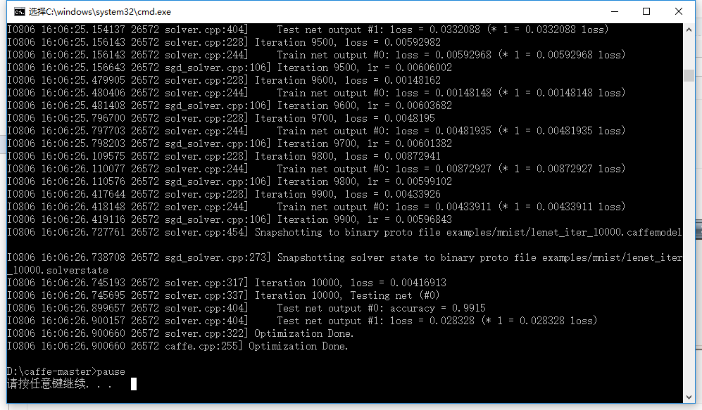
Based on the solver setting, we will print the training loss function every 100 iterations, and test the network every 500 iterations. You will see messages like this:

I1203 solver.cpp:204] Iteration 100, lr = 0.00992565
I1203 solver.cpp:66] Iteration 100, loss = 0.26044
...
I1203 solver.cpp:84] Testing net
I1203 solver.cpp:111] Test score #0: 0.9785
I1203 solver.cpp:111] Test score #1: 0.0606671

For each training iteration, lr is the learning rate of that iteration, and loss is the training function. For the output of the testing phase, score 0 is the accuracy, and score 1 is the testing loss function.

And after a few minutes, you are done!

I1203 solver.cpp:84] Testing net
I1203 solver.cpp:111] Test score #0: 0.9897
I1203 solver.cpp:111] Test score #1: 0.0324599
I1203 solver.cpp:126] Snapshotting to lenet_iter_10000
I1203 solver.cpp:133] Snapshotting solver state to lenet_iter_10000.solverstate
I1203 solver.cpp:78] Optimization Done.

The final model, stored as a binary protobuf file, is stored at

lenet_iter_10000

which you can deploy as a trained model in your application, if you are training on a real-world application dataset.

How to reduce the learning rate at fixed steps?

Look at lenet_multistep_solver.prototxt

3. 总结

通过前面博文的LeNet模型的使用，我们可以发现，使用caffe训练模型只需要以下几个步骤：

• 准备好数据
• 写好模型配置文件
• 写好优化配置文件
• 命令行执行