
利用RNN进行中文文本分类(数据集是复旦中文语料)
利用TfidfVectorizer进行中文文本分类(数据集是复旦中文语料)
1、训练词向量
数据预处理参考利用TfidfVectorizer进行中文文本分类(数据集是复旦中文语料) ,现在我们有了分词后的train_jieba.txt和test_jieba.txt,看一下部分内容:
fenci_path = '/content/drive/My Drive/NLP/dataset/Fudan/train_jieba.txt'
with open(fenci_path,'r',encoding='utf-8') as fp:
    i = 0
    lines = fp.readlines()
    for line in lines:
      print(line)
      i += 1
      if i == 10:
        break
每一篇文章的分词结果和标签都是一行,标签之间使用'\t'隔开。
由于之前只是简略的进行分词,没有过滤掉一些停用词,接下来还需要进行一些处理,我们之前已经建立了停用词文本:stopwords.txt,现在我们要使用它。
def clean():
  label_list = []
  content_list = []
  with open('/content/drive/My Drive/NLP/dataset/Fudan/train_jieba.txt','r',encoding='utf-8') as fp:
    lines = fp.readlines()
    for line in lines:
      tmp = line.strip().split("\t")
      content,label = tmp[0],tmp[1]
      label_list.append(label)
      out_list = []
      for word in content.strip().split(' '):
        if word not in stopwords_list and word != '':
          out_list.append(word)
        else:
          continue
      content_list.append(" ".join(out_list))
  return content_list,label_list
content_list,label_list = clean()
i = 0
for content,label in zip(content_list,label_list):
  print(content,label)
  i += 1
  if i == 10:
    break
确实是过滤掉了一些停用词,如果效果不好可以根据当前任务情况继续扩充停用词 ,这里就暂时到这了。
对训练集和测试集进行同样的清理后保存:
def save(content_list,label_list):
  path = '/content/drive/My Drive/NLP/dataset/Fudan/train_clean_jieba.txt'
  fp = open(path,'w',encoding='utf-8')
  for content,label in zip(content_list,label_list):
    fp.write(content+str(label)+'\n')
  fp.close()
save(content_list,label_list)
对测试集进行相同的操作时这一句 content,label = tmp[0],tmp[1] 出现了:list out of range
只需要多加一句:if len(tmp) == 2:过滤以下即可。
def clean():
  label_list = []
  content_list = []
  with open('/content/drive/My Drive/NLP/dataset/Fudan/test_jieba.txt','r',encoding='utf-8') as fp:
    lines = fp.readlines()
    for line in lines:
      tmp = line.strip().split("\t")
      if len(tmp) == 2:
        content,label = tmp[0],tmp[1]
      label_list.append(label)
      out_list = []
      for word in content.strip().split(' '):
        if word not in stopwords_list and word != '':
          out_list.append(word)
        else:
          continue
      content_list.append(" ".join(out_list))
  return content_list,label_list
content_list,label_list = clean()
def save(content_list,label_list):
  path = '/content/drive/My Drive/NLP/dataset/Fudan/test_clean_jieba.txt'
  fp = open(path,'w',encoding='utf-8')
  for content,label in zip(content_list,label_list):
    fp.write(content+'\t'+str(label)+'\n')
  fp.close()
save(content_list,label_list)
2、训练word2vec,构建词向量
我们新建一个data文件夹,然后将train_clean_jieba.txt和test_clean_jieba.txt放进去。这里word2vec的用法就不具体介绍了。
from gensim.models import Word2Vec
from gensim.models.word2vec import PathLineSentences
import multiprocessing
import os
import sys
import logging

# 日志信息输出
program = os.path.basename(sys.argv[0])
logger = logging.getLogger(program)
logging.basicConfig(format='%(asctime)s: %(levelname)s: %(message)s')
logging.root.setLevel(level=logging.INFO)
logger.info("running %s" % ' '.join(sys.argv))

# check and process input arguments
# if len(sys.argv) < 4:
#     print(globals()['__doc__'] % locals())
#     sys.exit(1)
# input_dir, outp1, outp2 = sys.argv[1:4]

# 训练模型
# 输入语料目录:PathLineSentences(input_dir)
# embedding size:100 共现窗口大小:5 去除出现次数5以下的词,多线程运行,迭代5次
model = Word2Vec(PathLineSentences('/content/drive/My Drive/NLP/dataset/Fudan/data/'),
                     size=100, window=5, min_count=5,
                     workers=multiprocessing.cpu_count(), iter=5)
model.save('/content/drive/My Drive/NLP/dataset/Fudan/Word2vec.w2v')
运行之后是这个样子:
2020-10-16 13:57:28,601: INFO: running /usr/local/lib/python3.6/dist-packages/ipykernel_launcher.py -f /root/.local/share/jupyter/runtime/kernel-52776eb8-5141-458e-8f04-3d3a0f11d46f.json
2020-10-16 13:57:28,606: INFO: reading directory /content/drive/My Drive/NLP/dataset/Fudan/data/
2020-10-16 13:57:28,608: INFO: files read into PathLineSentences:/content/drive/My Drive/NLP/dataset/Fudan/data/test_clean_jieba.txt
/content/drive/My Drive/NLP/dataset/Fudan/data/train_clean_jieba.txt
2020-10-16 13:57:28,610: INFO: collecting all words and their counts
2020-10-16 13:57:28,612: INFO: reading file /content/drive/My Drive/NLP/dataset/Fudan/data/test_clean_jieba.txt
/usr/local/lib/python3.6/dist-packages/smart_open/smart_open_lib.py:252: UserWarning: This function is deprecated, use smart_open.open instead. See the migration notes for details: https://github.com/RaRe-Technologies/smart_open/blob/master/README.rst#migrating-to-the-new-open-function
  'See the migration notes for details: %s' % _MIGRATION_NOTES_URL
2020-10-16 13:57:28,627: INFO: PROGRESS: at sentence #0, processed 0 words, keeping 0 word types
2020-10-16 13:57:33,897: INFO: reading file /content/drive/My Drive/NLP/dataset/Fudan/data/train_clean_jieba.txt
2020-10-16 13:57:34,040: INFO: PROGRESS: at sentence #10000, processed 18311769 words, keeping 440372 word types
2020-10-16 13:57:39,060: INFO: collected 584112 word types from a corpus of 35545042 raw words and 19641 sentences
2020-10-16 13:57:39,062: INFO: Loading a fresh vocabulary
2020-10-16 13:57:39,768: INFO: effective_min_count=5 retains 183664 unique words (31% of original 584112, drops 400448)
2020-10-16 13:57:39,769: INFO: effective_min_count=5 leaves 34810846 word corpus (97% of original 35545042, drops 734196)
2020-10-16 13:57:40,320: INFO: deleting the raw counts dictionary of 584112 items
2020-10-16 13:57:40,345: INFO: sample=0.001 downsamples 19 most-common words
2020-10-16 13:57:40,345: INFO: downsampling leaves estimated 33210825 word corpus (95.4% of prior 34810846)
2020-10-16 13:57:40,951: INFO: estimated required memory for 183664 words and 100 dimensions: 238763200 bytes
2020-10-16 13:57:40,952: INFO: resetting layer weights
2020-10-16 13:58:15,170: INFO: training model with 2 workers on 183664 vocabulary and 100 features, using sg=0 hs=0 sample=0.001 negative=5 window=5
2020-10-16 13:58:15,174: INFO: reading file /content/drive/My Drive/NLP/dataset/Fudan/data/test_clean_jieba.txt
2020-10-16 13:58:16,183: INFO: EPOCH 1 - PROGRESS: at 1.11% examples, 481769 words/s, in_qsize 3, out_qsize 0
最后会生成:

接下来我们要使用模型,然后查看词以及其对应的词向量:
from gensim.models import Word2Vec
model = Word2Vec.load('/content/drive/My Drive/NLP/dataset/Fudan/Word2vec.w2v')
#所有词的数目
print(len(model.wv.index2word))
word_vector_dict = {}
for word in model.wv.index2word:
  word_vector_dict[word] = list(model[word])
i = 0
for k,v in word_vector_dict.items():
  print(k,v)
  i += 1
  if i == 5:
    break
结果:
/usr/local/lib/python3.6/dist-packages/smart_open/smart_open_lib.py:252: UserWarning: This function is deprecated, use smart_open.open instead. See the migration notes for details: https://github.com/RaRe-Technologies/smart_open/blob/master/README.rst#migrating-to-the-new-open-function
  'See the migration notes for details: %s' % _MIGRATION_NOTES_URL
183664
/usr/local/lib/python3.6/dist-packages/ipykernel_launcher.py:7: DeprecationWarning: Call to deprecated `__getitem__` (Method will be removed in 4.0.0, use self.wv.__getitem__() instead).
  import sys
. [-2.8709345, -0.47548708, 0.86331373, 1.2737428, 2.3575406, 2.0570302, -0.53931403, 1.2613002, 0.5172711, -1.6461672, 1.3732913, 0.86122376, -0.21252058, 2.0552237, 0.9418685, 0.3278085, 0.588585, -0.7969468, -1.8978101, -0.43336996, -0.4861237, -0.25338736, -0.5043334, 0.6816521, 4.776381, 1.3428804, 1.9577577, 0.2862259, -1.3767976, 1.2107555, -0.21500991, 2.584977, -3.157238, -0.08438093, -1.4721884, -0.5101056, 0.39259034, 0.74332994, -0.6534138, 0.04722414, 2.2819524, 1.9146276, -0.13876201, -1.3124858, -1.2666191, 0.1447281, -0.5460836, 1.7340208, 0.5979215, -4.0311975, 0.11542667, -0.6193901, -0.058931056, 1.9952455, -0.8310607, -0.9370241, 0.2416995, -1.4236349, -0.41856983, -0.5497827, 1.2359228, 0.01779593, 0.9849501, 1.2311344, 1.8523129, 2.363041, 1.0974075, -1.2220355, 0.110876285, 0.17010106, -0.9745132, 1.1252304, 0.20266196, 1.6555228, -0.69005895, -0.15593, -2.6057267, 0.59146214, -0.29261357, 0.83551484, -2.1035368, 1.1904488, -1.0554912, -0.641594, 1.2142769, -1.4514563, 0.9756896, 0.52437824, -0.8486732, -3.358046, -0.69511414, 1.8128188, 0.45924014, -1.1814638, -0.48232678, -0.12257868, 0.23399891, -3.303544, -0.6949516, 0.5121446]
, [-2.618333, -1.8558567, 1.8535767, -0.21151228, 1.7623954, 4.3192573, 0.09128157, 1.5980599, 0.7076833, -1.7116284, 1.0046017, -0.15326972, 0.4059908, 0.9488417, 2.2387662, 0.20677945, -0.7107643, -2.758641, -0.3840812, 0.16083181, -2.1107125, 0.24038436, -1.2403657, 2.7272208, 1.9277251, 0.1489557, 2.1110923, 0.5919174, -2.1878436, 0.36604762, 0.31739056, 5.550043, -3.364542, 0.70963943, 0.13099277, -2.2344782, -0.39852622, -0.24567917, -1.3379095, -0.27352497, 1.3079535, -0.3681397, 1.2069534, -0.7798161, -0.18939576, -0.373316, -1.1903548, 1.2864754, -0.61407185, -3.171876, -1.2982743, 1.7416263, 0.73636365, 0.9905826, -0.3719811, 0.05626492, -2.6127703, 0.83886856, 0.66923296, 1.2502893, 0.9262052, 0.42174354, -1.484305, -0.17558077, 1.9593159, 4.8938365, 0.61336166, -1.0788211, -1.0862421, -0.5105872, -2.6575727, 2.091327, -0.23270625, 2.284086, -0.98763543, 0.28696263, -2.2600112, -3.2595506, 0.025764514, 1.3404137, -0.71168816, 2.2680438, 0.48311472, 0.36931905, 0.938186, -1.6107051, -0.15926446, 1.3209386, -0.801876, -2.303902, -0.436481, 0.8073558, 0.38733667, -0.26957598, -1.4267699, -0.8020603, 0.414129, -3.3372293, 0.6402213, -0.19667119]
) [-0.80750054, -0.6121455, -1.0710338, -2.9930687, 2.0432, 4.141169, -0.15709901, 0.81717527, -1.5162835, -3.1241925, -0.10446141, 1.010525, -3.1002233, 1.6662389, 0.9942944, 0.85855705, 2.0851238, -1.6842883, -2.9477723, -0.2876924, -0.6282387, -0.28349137, -3.1225855, 2.2486699, 1.2903367, 2.2274559, 0.27433106, 0.57094145, -1.1607213, -0.4642481, -1.0572903, 3.2884996, -1.2198547, -1.6459501, 0.67363816, -2.5827177, -0.25848988, -1.1222432, 0.21818976, 1.8232889, 2.8271437, -0.617807, -1.4015028, 1.2166779, -0.8353678, 0.34809938, -0.46445072, -0.084388316, 0.7031371, -4.1085744, -0.50515014, -3.1198754, 0.72745895, 1.4460654, 0.9307348, -2.758027, 0.018058121, -0.8535555, 0.6409112, 0.1882723, -1.1798013, 1.3632597, -0.1337653, 0.51510906, -0.5415601, 4.006427, -0.91912925, -3.4697065, -2.7071013, -0.6627828, -2.9176655, 1.0004271, 0.8123536, 2.1355457, -0.013824586, -0.10087594, 0.115427904, -0.46978354, 2.071482, 1.8447496, 0.99563545, 2.845259, 1.1902128, 0.02504066, 2.6136658, -0.6704431, -0.47580847, 1.1602222, 1.2428118, -2.3880181, -1.6264966, 0.74079543, -0.54774994, 1.0163826, -0.736786, -1.8922712, 0.5381837, -1.1004277, 0.33553576, 0.40247878]
( [-2.4204996, -1.0095057, 0.36723495, -1.9701287, 1.5028982, 1.0829349, -0.72509646, 1.0087173, -0.8471445, 0.21284652, -0.4341774, -0.9700405, -1.300372, 0.9491097, 3.350109, 1.4735373, 2.9339328, -0.3343834, -3.6445296, -0.41197056, -1.338803, 0.28331625, 0.10618747, -1.3739557, 1.1008664, 0.17741367, 0.45283958, 1.5100185, -1.7710751, 1.0186597, 0.7735381, 2.491264, 0.07328774, -1.1831408, -3.2152338, -2.5108373, -0.34185433, 0.34209073, -0.14207332, -2.194724, 1.0734048, -1.1285906, 1.9627889, -1.5373456, -1.9735036, 2.2119362, -0.21241511, 1.8747587, -0.67907304, -4.566279, -2.0092149, -1.3107775, 0.3573235, 0.9350223, 0.4996264, 1.6724535, -0.79917055, -0.14005652, 2.7869322, 0.80775166, 0.13976693, 0.5046433, -0.34996128, 0.3425343, 3.6427495, 2.3169396, -1.0229387, -4.0736656, 0.09746367, 0.79698503, -3.6760647, 0.53965265, -2.018294, 2.074562, -0.5203732, 0.06932237, -1.1419374, -1.2626162, 1.5128584, 1.1419917, -2.4901378, 3.0212705, 3.0879154, -1.0666283, 1.4316878, 0.25575432, 1.0118675, -0.210056, 1.5728005, -3.074708, -2.050965, 2.177831, -1.4306773, 0.5591415, -1.6649296, -2.479498, 0.27199566, -0.7439327, 1.065499, -1.7122517]
中 [-1.4137642, 0.07996469, -0.84706545, 0.9269082, -0.5876861, 0.9406654, -2.7666419, 0.013692471, 0.7948517, -3.7575817, -3.0255227, -0.1290994, 0.15024899, 1.7057111, -1.783816, 1.2594382, -0.80985075, 1.2856516, -1.1239803, 0.33939472, 1.7681189, 0.5220787, -3.093301, -0.72288835, -0.27703923, 0.6913874, -0.62614673, 0.16310164, 1.6016583, -0.9558958, -0.65395266, -0.81403816, -0.35800782, -1.6817136, 0.0038451876, 0.924515, 0.7525097, -0.55127585, -2.7082217, -0.5226547, 0.65330553, -0.13418457, -0.11833907, -4.0032573, -0.56922513, -1.323926, 0.097095534, 1.0593758, 0.48968402, -0.6643793, 1.4596446, -2.0395942, 2.7365487, -1.0603454, -0.54655385, -2.8474076, 0.3412293, 0.96139586, 0.9478409, 0.7041088, 4.2240176, -0.5293954, -3.0038583, -3.1062794, 0.55948454, 0.37824842, 0.13522537, 0.00925424, -1.3225565, 0.4190299, 0.57395566, -1.2779645, -0.6505884, 3.8218825, -1.2415665, -0.06736558, -1.7298794, 1.6446227, -1.0105107, -1.0007042, -0.7136034, 1.7795436, -0.8232877, 0.3342558, -1.9837192, -0.043689013, 0.4572051, 0.5139073, 1.9465048, 1.3884708, -1.18057, 3.5671742, -2.4114704, 1.324688, -0.14609453, -0.724388, 0.6249127, 0.600731, -2.1366022, 2.421635]
还是有一些标点符号没有去除,可以补充下停止词文本,这里就暂时这样了。
之后我们将词语保存在一个文件中,将对应的词向量保存在另一个文件中。
vocabulary_path = '/content/drive/My Drive/NLP/dataset/Fudan/vocabulary.txt'
vector_path = '/content/drive/My Drive/NLP/dataset/Fudan/vector.txt'
fp1 = open(vocabulary_path,'w',encoding='utf-8')
fp2 = open(vector_path,'w',encoding='utf-8')
for word in model.wv.index2word:
  fp1.write(word+'\n')
  vector_list = model[word]
  vector_str_list = [str(num) for num in vector_list]
  fp2.write(" ".join(vector_str_list)+"\n")
fp1.close()
fp2.close()
接着我们还需要进行一系列的转换操作:
import keras
#将词汇表中的单词映射成id
def word2id():
  vocabulary_path = '/content/drive/My Drive/NLP/dataset/Fudan/vocabulary.txt'
  fp1 = open(vocabulary_path,'r',encoding='utf-8')
  word2id_dict = {}
  for i,line in enumerate(fp1.readlines()):
    word2id_dict[line.strip()] = i
  print(word2id_dict)
  fp1.close()
  return word2id_dict
#得到文本内容及对应的标签
def get_content_label():
  data = '/content/drive/My Drive/NLP/dataset/Fudan/data/train_clean_jieba.txt'
  fp = open(data,'r',encoding='utf-8')
  content_list = []
  label_list = []
  for line in fp.readlines():
    line = line.strip().split('\t')
    if len(line) == 2:
      content_list.append(line[0])
      label_list.append(line[1])
  print(content_list[:5])
  print(label_list[:5])
  fp.close()
  return content_list,label_list
#得到标签对应的id
def get_label_id():
  label = '/content/drive/My Drive/NLP/dataset/Fudan/label.txt'
  label2id_dict = {}
  fp = open(label,'r',encoding='utf-8')
  for line in fp.readlines():
    line = line.strip().split('\t')
    label2id_dict[line[0]] = line[1]
  #print(label2id_dict)
  return label2id_dict
#将文本内容中的词替换成词对应的id,并设定文本的最大长度
#对标签进行one-hot编码
def process():
  max_length = 600
  data = '/content/drive/My Drive/NLP/dataset/Fudan/data/train_clean_jieba.txt'
  contents,labels = get_content_label()
  word_to_id = word2id()
  cat_to_id = get_label_id()
  data_id = []
  label_id = []
  for i in range(len(contents)):
    data_id.append([word_to_id[x] for x in contents[i] if x in word_to_id])
    label_id.append(cat_to_id[labels[i]])

  # 使用keras提供的pad_sequences来将文本pad为固定长度
  x_pad = keras.preprocessing.sequence.pad_sequences(data_id, max_length)
  y_pad = keras.utils.to_categorical(label_id, num_classes=len(cat_to_id))  # 将标签转换为one-hot表示
  return x_pad,y_pad
x_pad,y_pad = process()
print(x_pad[0])
print(y_pad[0])
print(len(x_pad),len(y_pad))
结果:
[  3464   2264   1227   1015   1844  34754   3464   2264   5781   2933
   1214   1499    519   2558    603  68784  50747   2706   1499   2127
   2558   3388   2912   1128   4617   1499   2127   3464   2264      4
   1499   2127   1244   5645  22020  55754   3464   2264   4419   5781
   2933   3464   2264   2558    603   1538     80   1104   1844      4
   1363   2821   5602   3464   2264   1244   5645   5308   2558    603
   1244   5645   1844  34754   3464   2264    238   1499   2558    603
   5602   5308   2127   2558    603    538    762   4437   2127   2558
    603   3388   2264   1024   1139    538   1818   1024   1139   1851
   1851   2327    139    929   1548    314    160   2602    482  10087
  13030   1730  40786   4754    139    562    366   6089      4    562
    160   2602     85   2433   5781     80    466   1139   1503   4453
   4617   1244   5645   3560   6058   3459      4    562    160   2602
   2558    603   3829   2517    410   4585   2558    603   3464   2264
   3848    423  11739   5645   3560   6058    431   3950   2127   1499
   2127     35    423  11739   5645    319   2558    603   1499   2127
   3773   4383      4   1503   1499   2558    603   1994   4419   1257
   1553    603    926   6065   1257   1553    603   1376    431   1538
     80   1090   2646   6506   7261    519   2558    603   1994   4419
   2456   2127   2558    603  20160   1553    603   1182   1090  16160
   4414   1137   1503   1844  34754      4    864  22754   1844  34754
   1730   3464   2264   2558    603  68784   3464   2264   2558    603
   5658  16754   6608   2558    603   3468   1776   4780  11201   5634
    429   1994   4419  38671   1730   3464   2264    755   2332  25839
    828   2558    603   3464   2264    429   3174    144   2840    429
   3174   1305   1164   2094  41825  33950      7      4    562   3464
   2264   3773   4383   7131    787   2264   3773   4383   3773   4383
   5326      8   1336  22020   2181   3464   2264   2558    603    915
    429  19614  11857   1844  34754    905   5372    429   3140   1116
   1371    780    858    780  22020  55754   3464   2264   2558    603
   4526   1032   1227   1015   1104   1844  17286   5308   2456   1104
   2193    429   3464   2264   2558    603   1336   3464   2264    755
   2558    603    755    888   2127   2558    603   1182   1090    139
   1499   2193    429   3464   2264   2558    603    220    201    144
   1844  34754   5223   3355    296   1321      0   1844   2602   5368
   4815    319    144    160   2602    915    429   2332   1996   1227
   1015   2114    384   2691  25814   2261    160   2602   1844  12894
   1996  20370  15958   1844  34754   4711   3994   1996      0   1844
  34754   1866   3241   6754    201   1305   2181   6754    201   2558
    603   2558    603   2193    429   2127   1090   4617   4982   2706
   1025   3119  10028   3464   2264   2558    603   1116    160   1182
   1090    950    384   1215  26769 116663    160   2602   1996    864
   2578   1864   5223    431  19429   3355    296   2578   1864   1851
   1851   2327   5223      0   1844  34754    238   2433   3464   2264
    458  39604    787    395   8527  30953    519   1090   4617   1321
    201   3119   2710   1321    201    519   1321    201   2558    603
   1321    201   1844  10087      0   1844  34754   1540    431    861
    562    787   1844    864     10   1411    787   2264   9301    519
  58253  13086   8527   3560   5648   3464   2264  10478   2181   1844
  34754      4      0   1844  34754     85   1077   2578   1864   1548
   8068   2578   1864      4    562    787   2264   1692   1938   2924
   1692   3837   2181   3683   7285     35   1844  34754    864    238
   1499    139    519   2806   1321    562   2236    301    395  50747
   2706   2574    429     35    254   2806   1321   1227    176   2574
    429    562    731   2281    139   1127   4668   3459    716   1548
   8068   2578   1864   2927   1636   2400   1851    139  14986   3773
  12279     80   3275   8128   2033   1723   7131    867   3468   2790
   1938  22337   2895  32268   2790   1723   1938  22337   2067   4914
   1723   1938  22337      7   3812   8246   4899   4178   8553   8595
   5487   1553    731   9237  45100    482    429   2684   1221      8]
[0. 0. 0. 0. 0. 0. 0. 0. 0. 1. 0. 0. 0. 0. 0. 0. 0. 0. 0. 0.]
9803 9803
最后我们再定义一个将数据制作成batch的操作:
def batch_iter(x, y, batch_size=64):
    """生成批次数据"""
    data_len = len(x)
    num_batch = int((data_len - 1) / batch_size) + 1

    indices = np.random.permutation(np.arange(data_len))
    x_shuffle = x[indices]
    y_shuffle = y[indices]

    for i in range(num_batch):
        start_id = i * batch_size
        end_id = min((i + 1) * batch_size, data_len)
        yield x_shuffle[start_id:end_id], y_shuffle[start_id:end_id]
3、ternsorflow中的RNN
RNN在tensorflow中有静态RNN,动态RNN之分。两者差异挺大,我们在使用tensorflow进行RNN实践时,主要注意以下几点:
- 静态RNN一般需要将所有句子padding成等长处理,这点与TextCNN一样的,但动态rnn稍显灵活一点,动态RNN中,只要一个batch中的所有句子等长就可以;
- 静态RNN的输入与输出是list或二维张量;动态RNN中输入输出的是三维张量,相对与TextCNN,少了一维;
- 静态RNN生成过程所需的时间更长,网络所占内存会更大,但模型中会带有每个序列的中间信息,利于调试;动态RNN生成过程所需时间相对少,所占内存相对更小,但模型中只有最后的状态。
本文介绍使用动态RNN进行文本分类。
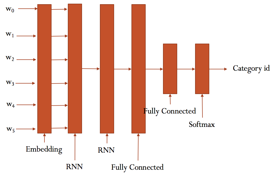
(1)我们首先要定义模型
class TRNNConfig(object):
    """RNN配置参数"""

    # 模型参数
    embedding_dim = 100      # 词向量维度
    seq_length = 600        # 序列长度
    num_classes = 20        # 类别数
    vocab_size = 183664       # 词汇总数

    num_layers= 2           # 隐藏层层数
    hidden_dim = 128        # 隐藏层神经元
    rnn = 'gru'             # lstm 或 gru

    dropout_keep_prob = 0.8 # dropout保留比例
    learning_rate = 1e-3    # 学习率

    batch_size = 128         # 每批训练大小
    num_epochs = 10         # 总迭代轮次

    print_per_batch = 20    # 每多少轮输出一次结果
    save_per_batch = 10      # 每多少轮存入tensorboard


class TextRNN(object):
    """文本分类,RNN模型"""
    def __init__(self, config):
        self.config = config

        # 三个待输入的数据
        self.input_x = tf.placeholder(tf.int32, [None, self.config.seq_length], name='input_x')
        self.input_y = tf.placeholder(tf.float32, [None, self.config.num_classes], name='input_y')
        self.keep_prob = tf.placeholder(tf.float32, name='keep_prob')

        self.rnn()

    def rnn(self):
        """rnn模型"""

        def lstm_cell():   # lstm核
            return tf.contrib.rnn.BasicLSTMCell(self.config.hidden_dim, state_is_tuple=True)

        def gru_cell():  # gru核
            return tf.contrib.rnn.GRUCell(self.config.hidden_dim)

        def dropout(): # 为每一个rnn核后面加一个dropout层
            if (self.config.rnn == 'lstm'):
                cell = lstm_cell()
            else:
                cell = gru_cell()
            return tf.contrib.rnn.DropoutWrapper(cell, output_keep_prob=self.keep_prob)

        # 词向量映射
        with tf.device('/cpu:0'):
            embedding = tf.get_variable('embedding', [self.config.vocab_size, self.config.embedding_dim])
            embedding_inputs = tf.nn.embedding_lookup(embedding, self.input_x)

        with tf.name_scope("rnn"):
            # 多层rnn网络
            cells = [dropout() for _ in range(self.config.num_layers)]
            rnn_cell = tf.contrib.rnn.MultiRNNCell(cells, state_is_tuple=True)

            _outputs, _ = tf.nn.dynamic_rnn(cell=rnn_cell, inputs=embedding_inputs, dtype=tf.float32)
            last = _outputs[:, -1, :]  # 取最后一个时序输出作为结果

        with tf.name_scope("score"):
            # 全连接层,后面接dropout以及relu激活
            fc = tf.layers.dense(last, self.config.hidden_dim, name='fc1')
            fc = tf.contrib.layers.dropout(fc, self.keep_prob)
            fc = tf.nn.relu(fc)

            # 分类器
            self.logits = tf.layers.dense(fc, self.config.num_classes, name='fc2')
            self.y_pred_cls = tf.argmax(tf.nn.softmax(self.logits), 1)  # 预测类别

        with tf.name_scope("optimize"):
            # 损失函数,交叉熵
            cross_entropy = tf.nn.softmax_cross_entropy_with_logits(logits=self.logits, labels=self.input_y)
            self.loss = tf.reduce_mean(cross_entropy)
            # 优化器
            self.optim = tf.train.AdamOptimizer(learning_rate=self.config.learning_rate).minimize(self.loss)

        with tf.name_scope("accuracy"):
            # 准确率
            correct_pred = tf.equal(tf.argmax(self.input_y, 1), self.y_pred_cls)
            self.acc = tf.reduce_mean(tf.cast(correct_pred, tf.float32))
模型大致结构如下:
(2)定义一些辅助函数
def evaluate(sess, x_, y_):
    """评估在某一数据上的准确率和损失"""
    data_len = len(x_)
    batch_eval = batch_iter(x_, y_, 128)
    total_loss = 0.0
    total_acc = 0.0
    for x_batch, y_batch in batch_eval:
        batch_len = len(x_batch)
        feed_dict = feed_data(x_batch, y_batch, 1.0)
        loss, acc = sess.run([model.loss, model.acc], feed_dict=feed_dict)
        total_loss += loss * batch_len
        total_acc += acc * batch_len

    return total_loss / data_len, total_acc / data_len

def get_time_dif(start_time):
    """获取已使用时间"""
    end_time = time.time()
    time_dif = end_time - start_time
    return timedelta(seconds=int(round(time_dif)))


def feed_data(x_batch, y_batch, keep_prob):
    feed_dict = {
        model.input_x: x_batch,
        model.input_y: y_batch,
        model.keep_prob: keep_prob
    }
    return feed_dict
(3)定义训练主函数
def train():
    print("Configuring TensorBoard and Saver...")
    # 配置 Tensorboard,重新训练时,请将tensorboard文件夹删除,不然图会覆盖
    tensorboard_dir = 'tensorboard/textrnn'
    if not os.path.exists(tensorboard_dir):
        os.makedirs(tensorboard_dir)

    tf.summary.scalar("loss", model.loss)
    tf.summary.scalar("accuracy", model.acc)
    merged_summary = tf.summary.merge_all()
    writer = tf.summary.FileWriter(tensorboard_dir)

    save_dir = 'checkpoints/textrnn'
    save_path = os.path.join(save_dir, 'best_validation')  # 最佳验证结果保存路径
    # 配置 Saver
    saver = tf.train.Saver()
    if not os.path.exists(save_dir):
        os.makedirs(save_dir)

    print("Loading training and validation data...")
    # 载入训练集与验证集
    start_time = time.time()
    train_dir = '/content/drive/My Drive/NLP/dataset/Fudan/data/train_clean_jieba.txt'
    val_dir = '/content/drive/My Drive/NLP/dataset/Fudan/data/test_clean_jieba.txt'
    x_train, y_train = process(train_dir, config.seq_length)
    x_val, y_val = process(val_dir, config.seq_length)
    time_dif = get_time_dif(start_time)
    print("Time usage:", time_dif)

    # 创建session
    session = tf.Session()
    session.run(tf.global_variables_initializer())
    writer.add_graph(session.graph)

    print('Training and evaluating...')
    start_time = time.time()
    total_batch = 0  # 总批次
    best_acc_val = 0.0  # 最佳验证集准确率
    last_improved = 0  # 记录上一次提升批次
    require_improvement = 1000  # 如果超过1000轮未提升,提前结束训练

    flag = False
    for epoch in range(config.num_epochs):
        print('Epoch:', epoch + 1)
        batch_train = batch_iter(x_train, y_train, config.batch_size)
        for x_batch, y_batch in batch_train:
            feed_dict = feed_data(x_batch, y_batch, config.dropout_keep_prob)

            if total_batch % config.save_per_batch == 0:
                # 每多少轮次将训练结果写入tensorboard scalar
                s = session.run(merged_summary, feed_dict=feed_dict)
                writer.add_summary(s, total_batch)

            if total_batch % config.print_per_batch == 0:
                # 每多少轮次输出在训练集和验证集上的性能
                feed_dict[model.keep_prob] = 1.0
                loss_train, acc_train = session.run([model.loss, model.acc], feed_dict=feed_dict)
                loss_val, acc_val = evaluate(session, x_val, y_val)  # todo

                if acc_val > best_acc_val:
                    # 保存最好结果
                    best_acc_val = acc_val
                    last_improved = total_batch
                    saver.save(sess=session, save_path=save_path)
                    improved_str = '*'
                else:
                    improved_str = ''

                time_dif = get_time_dif(start_time)
                msg = 'Iter: {0:>6}, Train Loss: {1:>6.2}, Train Acc: {2:>7.2%},' \
                      + ' Val Loss: {3:>6.2}, Val Acc: {4:>7.2%}, Time: {5} {6}'
                print(msg.format(total_batch, loss_train, acc_train, loss_val, acc_val, time_dif, improved_str))

            feed_dict[model.keep_prob] = config.dropout_keep_prob
            session.run(model.optim, feed_dict=feed_dict)  # 运行优化
            total_batch += 1

            if total_batch - last_improved > require_improvement:
                # 验证集正确率长期不提升,提前结束训练
                print("No optimization for a long time, auto-stopping...")
                flag = True
                break  # 跳出循环
        if flag:  # 同上
            break
if __name__ == '__main__':
  print('Configuring RNN model...')
  config = TRNNConfig()
  model = TextRNN(config)
  train()
运行部分结果:
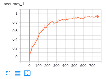
Epoch: 8
Iter:    540, Train Loss:   0.25, Train Acc:  92.19%, Val Loss:   0.62, Val Acc:  83.12%, Time: 0:22:00
Iter:    560, Train Loss:   0.28, Train Acc:  91.41%, Val Loss:   0.61, Val Acc:  84.18%, Time: 0:22:48
Iter:    580, Train Loss:   0.25, Train Acc:  91.41%, Val Loss:   0.59, Val Acc:  84.61%, Time: 0:23:36 *
Iter:    600, Train Loss:   0.39, Train Acc:  89.06%, Val Loss:   0.62, Val Acc:  83.94%, Time: 0:24:24
Epoch: 9
Iter:    620, Train Loss:   0.17, Train Acc:  95.31%, Val Loss:   0.59, Val Acc:  84.75%, Time: 0:25:12 *
Iter:    640, Train Loss:   0.24, Train Acc:  92.97%, Val Loss:   0.57, Val Acc:  85.21%, Time: 0:26:00 *
Iter:    660, Train Loss:   0.23, Train Acc:  94.53%, Val Loss:   0.61, Val Acc:  83.84%, Time: 0:26:47
Iter:    680, Train Loss:   0.33, Train Acc:  90.62%, Val Loss:    0.6, Val Acc:  85.02%, Time: 0:27:35
Epoch: 10
Iter:    700, Train Loss:   0.23, Train Acc:  92.97%, Val Loss:   0.63, Val Acc:  83.92%, Time: 0:28:22
Iter:    720, Train Loss:   0.29, Train Acc:  92.97%, Val Loss:   0.59, Val Acc:  85.37%, Time: 0:29:10 *
Iter:    740, Train Loss:   0.13, Train Acc:  96.09%, Val Loss:   0.59, Val Acc:  84.92%, Time: 0:29:57
Iter:    760, Train Loss:   0.32, Train Acc:  91.41%, Val Loss:   0.62, Val Acc:  84.72%, Time: 0:30:44
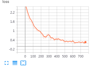
在tensorboard可视化结果:

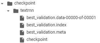
同时会生成保存的文件:
进行测试,这里我们的测试集和验证集是同样的:
def test():
  print("Loading test data...")
  start_time = time.time()
  test_dir = '/content/drive/My Drive/NLP/dataset/Fudan/data/test_clean_jieba.txt'
  x_test, y_test = process(test_dir, config.seq_length)
  save_path = 'checkpoint/textrnn/best_validation'
  session = tf.Session()
  session.run(tf.global_variables_initializer())
  saver = tf.train.Saver()
  saver.restore(sess=session, save_path=save_path)  # 读取保存的模型

  print('Testing...')
  loss_test, acc_test = evaluate(session, x_test, y_test)
  msg = 'Test Loss: {0:>6.2}, Test Acc: {1:>7.2%}'
  print(msg.format(loss_test, acc_test))

  batch_size = 128
  data_len = len(x_test)
  num_batch = int((data_len - 1) / batch_size) + 1

  y_test_cls = np.argmax(y_test, 1)
  y_pred_cls = np.zeros(shape=len(x_test), dtype=np.int32)  # 保存预测结果
  for i in range(num_batch):  # 逐批次处理
      start_id = i * batch_size
      end_id = min((i + 1) * batch_size, data_len)
      feed_dict = {
          model.input_x: x_test[start_id:end_id],
          model.keep_prob: 1.0
      }
      y_pred_cls[start_id:end_id] = session.run(model.y_pred_cls, feed_dict=feed_dict)

  # 评估
  print("Precision, Recall and F1-Score...")
  categories = get_label_id().values()
  print(metrics.classification_report(y_test_cls, y_pred_cls, target_names=categories))

  # 混淆矩阵
  print("Confusion Matrix...")
  cm = metrics.confusion_matrix(y_test_cls, y_pred_cls)
  print(cm)

  time_dif = get_time_dif(start_time)
  print("Time usage:", time_dif)
if __name__ == '__main__':
  print('Configuring RNN model...')
  config = TRNNConfig()
  model = TextRNN(config)
  test()
结果:这里9833是因为最后面多出了一行空行
Test Loss:   0.61, Test Acc:  84.53%
Precision, Recall and F1-Score...
/usr/local/lib/python3.6/dist-packages/sklearn/metrics/_classification.py:1272: UndefinedMetricWarning: Precision and F-score are ill-defined and being set to 0.0 in labels with no predicted samples. Use `zero_division` parameter to control this behavior.
  _warn_prf(average, modifier, msg_start, len(result))
              precision    recall  f1-score   support

           0       0.00      0.00      0.00        61
           1       0.87      0.90      0.88      1022
           2       0.28      0.32      0.30        59
           3       0.87      0.91      0.89      1254
           4       0.60      0.40      0.48        52
           5       0.74      0.88      0.80      1026
           6       0.95      0.94      0.94      1358
           7       0.50      0.02      0.04        45
           8       0.40      0.24      0.30        76
           9       0.84      0.88      0.86       742
          10       0.60      0.09      0.15        34
          11       0.00      0.00      0.00        28
          12       0.91      0.92      0.92      1218
          13       0.85      0.85      0.85       642
          14       0.36      0.12      0.18        33
          15       0.44      0.15      0.22        27
          16       0.88      0.88      0.88      1601
          17       0.27      0.45      0.34        53
          18       0.33      0.12      0.17        34
          19       0.65      0.52      0.58       468

    accuracy                           0.85      9833
   macro avg       0.57      0.48      0.49      9833
weighted avg       0.83      0.85      0.84      9833

Confusion Matrix...
[[   0    3    2   43    0    3    0    0    1    1    0    0    0    1
     0    0    2    0    0    5]
 [   0  916    0   13    0    6    0    0    0    1    0    0   21    0
     0    0   49    8    2    6]
 [   0    2   19    2    1    1    3    0    1    0    0    0    5    5
     2    2    1   13    1    1]
 [   0    8    1 1147    0   45    1    0    2    7    0    0    4    5
     0    0   12    3    1   18]
 [   0    2    1    5   21    4    2    0    1    3    0    0    2    1
     0    0    6    2    0    2]
 [   0    4    0   23    1  898    0    0    3   13    0    0    0    0
     0    0   67    0    1   16]
 [   0    0    1    9    0    1 1278    0    0    8    1    0    6   46
     0    0    7    1    0    0]
 [   0    0    1    9    0   16    1    1    0   11    0    0    0    0
     0    1    2    0    0    3]
 [   0    1    3    7    0   23    1    0   18    2    0    0    0    2
     1    0    1    3    0   14]
 [   0    0    0    2    2   29    2    0    1  651    1    0    0    0
     0    0    3    1    0   50]
 [   0    0    0    1    0    4    0    1    2   15    3    0    0    0
     0    0    2    1    0    5]
 [   0    0    0    3    0    1    4    0    0    0    0    0    5    6
     0    0    6    3    0    0]
 [   0   32    5    5    3    0   15    0    0    0    0    0 1117   13
     1    1   21    3    2    0]
 [   0    6   15    8    3    0   33    0    4    1    0    0   18  546
     0    0    0    8    0    0]
 [   0    2    2    0    1    2    0    0    0    1    0    0   11    6
     4    0    3    0    0    1]
 [   0    0    0    2    0    1    8    0    2    0    0    0    2    6
     0    4    1    0    0    1]
 [   0   59    3   21    1   55    3    0    3    2    0    0   25    0
     2    0 1416    5    1    5]
 [   0    7    9    4    0    1    0    0    3    0    0    0    0    0
     0    0    2   24    0    3]
 [   0    4    5    0    1    2    0    0    1    0    0    0    5    0
     1    0    2    8    4    1]
 [   0    4    1   15    1  118    0    0    3   61    0    0    0    2
     0    1   10    7    0  245]]
Time usage: 0:01:01
上面的模型是没有加入到我们预先训练好的词向量的,接下来,我们要将自己的词向量导入到模型中,再进行训练。
4、将词向量加入到网络中
首先我们需要对词向量进行处理:生成一个词嵌入,然后将词向量赋值给对应的位置
import numpy as np
def export_word2vec_vectors():
  word2vec_dir = '/content/drive/My Drive/NLP/dataset/Fudan/vector.txt'
  trimmed_filename = '/content/drive/My Drive/NLP/dataset/Fudan/vector_word.npz'
  file_r = open(word2vec_dir, 'r', encoding='utf-8')
  #(183664,100)
  lines = file_r.readlines()
  embeddings = np.zeros([183664, 100])
  for i,vec in enumerate(lines):
    vec = vec.strip().split(" ")
    vec = np.asarray(vec,dtype='float32')
    embeddings[i] = vec
  np.savez_compressed(trimmed_filename, embeddings=embeddings)
export_word2vec_vectors()
之后用这种方式进行读取:
def get_training_word2vec_vectors(filename):
  with np.load(filename) as data:
      return data["embeddings"]
接下来看看我们需要修改的地方:
在模型配置文件中加入:
    pre_trianing = None
    vector_word_npz = '/content/drive/My Drive/NLP/dataset/Fudan/vector_word.npz'
在模型中修改:
#embedding = tf.get_variable('embedding', [self.config.vocab_size, self.config.embedding_dim])
            embedding = tf.get_variable("embeddings", shape=[self.config.vocab_size, self.config.embedding_dim],
                                             initializer=tf.constant_initializer(self.config.pre_trianing))
            embedding_inputs = tf.nn.embedding_lookup(embedding, self.input_x)
在main中修改:
if __name__ == '__main__':
  print('Configuring RNN model...')
  config = TRNNConfig()
  config.pre_trianing = get_training_word2vec_vectors(config.vector_word_npz)
  model = TextRNN(config)
  train()
然后我们运行:
Epoch: 8
Iter:    540, Train Loss:   0.17, Train Acc:  92.97%, Val Loss:   0.44, Val Acc:  87.80%, Time: 0:22:14
Iter:    560, Train Loss:   0.17, Train Acc:  96.09%, Val Loss:   0.39, Val Acc:  89.10%, Time: 0:23:04 *
Iter:    580, Train Loss:   0.14, Train Acc:  94.53%, Val Loss:    0.4, Val Acc:  88.71%, Time: 0:23:51
Iter:    600, Train Loss:   0.16, Train Acc:  92.97%, Val Loss:   0.39, Val Acc:  89.10%, Time: 0:24:37
Epoch: 9
Iter:    620, Train Loss:   0.14, Train Acc:  93.75%, Val Loss:    0.4, Val Acc:  88.78%, Time: 0:25:25
Iter:    640, Train Loss:   0.16, Train Acc:  96.09%, Val Loss:   0.42, Val Acc:  88.67%, Time: 0:26:13
Iter:    660, Train Loss:   0.13, Train Acc:  96.09%, Val Loss:   0.42, Val Acc:  88.95%, Time: 0:26:59
Iter:    680, Train Loss:   0.18, Train Acc:  94.53%, Val Loss:    0.4, Val Acc:  89.17%, Time: 0:27:47 *
Epoch: 10
Iter:    700, Train Loss:   0.19, Train Acc:  94.53%, Val Loss:   0.43, Val Acc:  89.06%, Time: 0:28:35
Iter:    720, Train Loss:  0.046, Train Acc:  98.44%, Val Loss:    0.4, Val Acc:  89.72%, Time: 0:29:22 *
Iter:    740, Train Loss:   0.11, Train Acc:  96.09%, Val Loss:   0.44, Val Acc:  88.86%, Time: 0:30:10
Iter:    760, Train Loss:  0.059, Train Acc:  97.66%, Val Loss:   0.39, Val Acc:  89.47%, Time: 0:30:57
再进行测试:
Test Loss:    0.4, Test Acc:  89.72%
Precision, Recall and F1-Score...
              precision    recall  f1-score   support

           0       0.48      0.38      0.42        61
           1       0.93      0.91      0.92      1022
           2       0.58      0.51      0.54        59
           3       0.95      0.93      0.94      1254
           4       0.75      0.40      0.53        52
           5       0.87      0.91      0.89      1026
           6       0.93      0.98      0.96      1358
           7       0.41      0.31      0.35        45
           8       0.64      0.57      0.60        76
           9       0.89      0.91      0.90       742
          10       0.57      0.12      0.20        34
          11       0.36      0.18      0.24        28
          12       0.94      0.95      0.95      1218
          13       0.93      0.92      0.92       642
          14       0.42      0.15      0.22        33
          15       0.33      0.07      0.12        27
          16       0.90      0.94      0.92      1601
          17       0.56      0.60      0.58        53
          18       0.36      0.15      0.21        34
          19       0.75      0.74      0.75       468

    accuracy                           0.90      9833
   macro avg       0.68      0.58      0.61      9833
weighted avg       0.89      0.90      0.89      9833

Confusion Matrix...
[[  23    0    0   17    0    2    1    1    0    5    0    0    2    1
     0    0    3    6    0    0]
 [   0  926    0    0    0    3    0    0    0    0    0    0    7    1
     0    0   72    1    0   12]
 [   0    1   30    0    1    0   13    0    0    0    0    1    0    5
     0    1    6    1    0    0]
 [   8    6    0 1165    0   21    4    0    1   14    0    0    8    3
     0    0    8    3    0   13]
 [   0    0    4    0   21    5    4    0    3    0    0    1    4    0
     0    1    9    0    0    0]
 [   3    5    0   12    2  932    0    6   11    4    0    0    3    0
     0    0   28    1    0   19]
 [   0    0    1    1    0    0 1336    0    0    0    0    3    3   12
     0    0    2    0    0    0]
 [   3    0    0   10    0    8    0   14    0    6    0    0    0    1
     0    0    1    0    0    2]
 [   1    1    2    0    0   15    2    0   43    0    0    0    0    3
     0    0    0    8    0    1]
 [   0    0    1    2    1    0    2    5    1  675    3    0    0    0
     0    0    1    0    0   51]
 [   0    0    0    2    0    2    0    4    2   10    4    0    0    0
     0    0    1    0    0    9]
 [   0    0    1    1    0    0    9    0    0    0    0    5    0    6
     0    1    4    1    0    0]
 [   1   14    0    0    0    2   13    0    2    0    0    0 1161    5
     0    0   17    0    3    0]
 [   0    6    1    3    0    0   28    0    0    1    0    0   12  589
     0    0    1    1    0    0]
 [   0    1    2    0    0    1    0    0    0    0    0    1   14    2
     5    0    4    0    3    0]
 [   0    0    6    0    0    1   12    0    1    0    0    1    0    2
     0    2    2    0    0    0]
 [   1   27    3    4    2   32    3    3    0    0    0    0    4    0
     1    1 1509    3    3    5]
 [   8    2    0    3    1    1    0    0    0    0    0    1    2    0
     1    0    2   32    0    0]
 [   0    1    1    0    0    0    1    0    0    0    0    1   12    2
     5    0    6    0    5    0]
 [   0    4    0    5    0   48    4    1    3   46    0    0    0    4
     0    0    8    0    0  345]]
Time usage: 0:01:02
使用了我们预先训练的词向量之后,发现比随机生成的词向量相比,确实能够提升网络的性能。
最后做个总结:
使用RNN进行文本分类的过程如下:
- 获取数据;
- 无论数据是什么格式的,我们需要对其进行分词(去掉停用词)可以根据频率进行选择前N个词(可选);
- 我们需要所有词,并对它们进行编号;
- 训练词向量(可选),要将训练好的向量和词编号进行对应;
- 将数据集中的句子中的每个词用编号代替,对标签也进行编号,让标签和标签编号对应;
- 文本可使用keras限制它的最大长度,标签进行onehot编码;
- 读取数据集(文本和标签),然后构建batchsize
- 搭建模型并进行训练和测试;
至此从数据的处理到文本分类的整个流程就已经全部完成了,接下来还是对该数据集,使用CNN进行训练和测试。欢迎关注我的微信公众号-西西嘛呦,它不橡博客园发表那样长篇大论的文章,只希望能够带给你有用的知识。
参考:
https://www.jianshu.com/p/cd9563a3f6c9
https://github.com/cjymz886/text-cnn
https://github.com/gaussic/text-classification-cnn-rnn/

 浙公网安备 33010602011771号