
量化交易——双均线策略(金叉死叉)
一、双均线概念
均线:对于每一个交易日,都可以计算出前N天的移动平均值,然后把这些平均值连起来,成为一条线,就叫做N日移动平均线。移动平均线常用线有5日、10日、30日、60日、120日的指标。
5日和10日的是短线操作参照指标,称作日均线指标;
30日和60日的是中期均线指标,称作季均线指标;
120日和240日的是长期均线指标,称作年均线指标。
金叉:短期均线上穿长期均线,买入信号。
死叉:短期均线下穿长期均线,卖出信号。
交易策略:金叉买入,死叉卖出。
二、金叉死叉交易练习
1、使用tushare包获取某股票的历史行情
import numpy as np
import pandas as pd
import matplotlib.pyplot as plt    # Python绘图和数据可视化的工具包
import tushare as ts


ts.get_k_data("601318", start="2004-01-30").to_csv('601318.csv')
df = pd.read_csv('601318.csv', index_col="date", parse_dates=['date'])[['open', 'close', 'high', 'low']]
print(df)
"""
              open   close    high     low
date
2007-03-01  21.254  19.890  21.666  19.469
2007-03-02  19.979  19.728  20.166  19.503
...            ...     ...     ...     ...
2020-01-22  85.000  85.220  85.480  83.830
2020-01-23  84.010  83.490  84.560  82.480

[3076 rows x 4 columns]
"""
2、使用pandas包计算该股票历史数据的5日和30均线
5日均线则前4天没有均线,30日均线则前29天没有均线。
(1)普通方法
df['ma5'] = np.nan     # 创建5日均值列
df['ma30'] = np.nan    # 创建30日均值列
print(df)
"""
              open   close    high     low  ma5  ma30
date
2007-03-01  21.254  19.890  21.666  19.469  NaN   NaN
2007-03-02  19.979  19.728  20.166  19.503  NaN   NaN
...            ...     ...     ...     ...  ...   ...
2020-01-22  85.000  85.220  85.480  83.830  NaN   NaN
2020-01-23  84.010  83.490  84.560  82.480  NaN   NaN
"""
for i in range(4, len(df)):    # 从第五个到最后一个
    # 当天和前四天的收盘价的平均值为5日均线值
    df.loc[df.index[i], 'ma5'] = df["close"][i-4:i+1].mean()   # i=4是第五天,[0,5]
print(df)
"""
              open   close    high     low      ma5  ma30
date
2007-03-01  21.254  19.890  21.666  19.469      NaN   NaN
2007-03-02  19.979  19.728  20.166  19.503      NaN   NaN
2007-03-05  19.545  18.865  19.626  18.504      NaN   NaN
2007-03-06  18.704  19.235  19.554  18.597      NaN   NaN
2007-03-07  19.252  19.758  19.936  19.090  19.4952   NaN
...            ...     ...     ...     ...      ...   ...
2020-01-23  84.010  83.490  84.560  82.480  85.6320   NaN
"""

for i in range(29, len(df)):    # 从第30个到最后一个
    # 当天和前29天的收盘价的平均值为30日均线值
    df.loc[df.index[i], 'ma30'] = df["close"][i-29:i+1].mean()
print(df)
"""
              open   close    high     low      ma5       ma30
date
2007-03-01  21.254  19.890  21.666  19.469      NaN        NaN
2007-03-02  19.979  19.728  20.166  19.503      NaN        NaN
2007-03-05  19.545  18.865  19.626  18.504      NaN        NaN
2007-03-06  18.704  19.235  19.554  18.597      NaN        NaN
2007-03-07  19.252  19.758  19.936  19.090  19.4952        NaN
...            ...     ...     ...     ...      ...        ...
2020-01-17  86.150  86.250  86.900  85.850  86.1780  85.292333
2020-01-20  88.300  87.600  88.700  87.350  86.4080  85.387667
2020-01-21  87.000  85.600  87.290  85.600  86.1620  85.452667
2020-01-22  85.000  85.220  85.480  83.830  86.0440  85.507000
2020-01-23  84.010  83.490  84.560  82.480  85.6320  85.488667
"""
(2)简单方法
df['ma5'] = df['close'].rolling(5).mean()
df['ma30'] = df['close'].rolling(30).mean()
print(df)
"""
              open   close    high     low      ma5       ma30
date
2007-03-01  21.254  19.890  21.666  19.469      NaN        NaN
2007-03-02  19.979  19.728  20.166  19.503      NaN        NaN
2007-03-05  19.545  18.865  19.626  18.504      NaN        NaN
2007-03-06  18.704  19.235  19.554  18.597      NaN        NaN
2007-03-07  19.252  19.758  19.936  19.090  19.4952        NaN
...            ...     ...     ...     ...      ...        ...
2020-01-17  86.150  86.250  86.900  85.850  86.1780  85.292333
2020-01-20  88.300  87.600  88.700  87.350  86.4080  85.387667
2020-01-21  87.000  85.600  87.290  85.600  86.1620  85.452667
2020-01-22  85.000  85.220  85.480  83.830  86.0440  85.507000
2020-01-23  84.010  83.490  84.560  82.480  85.6320  85.488667
"""
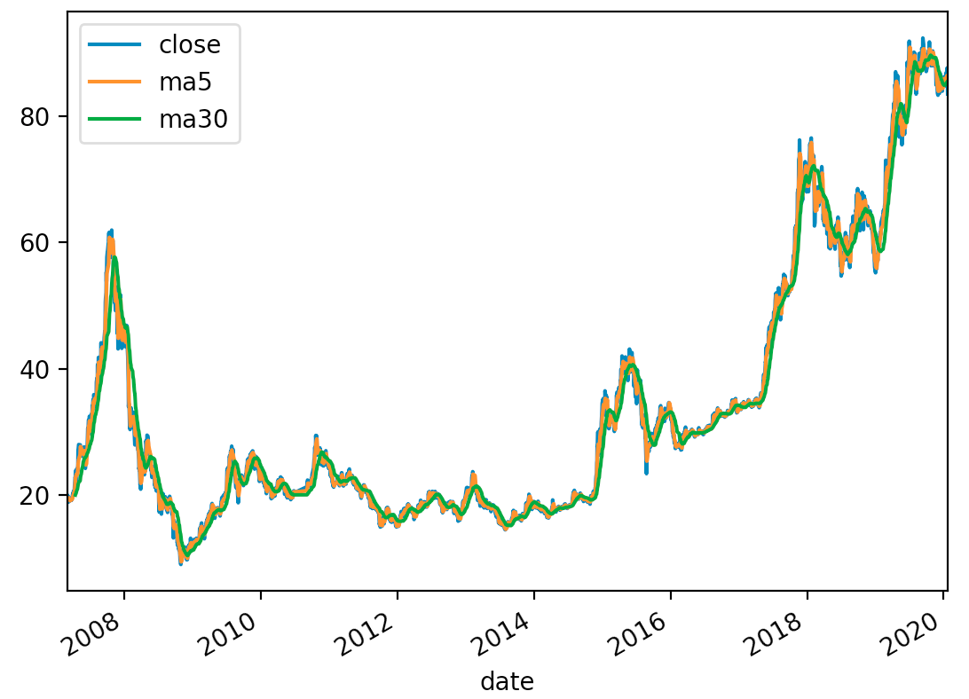
3、使用matplotlib包可视化历史数据的收盘价和两条均线
df[['close', 'ma5', 'ma30']].plot()
plt.show()
运行后显示效果:
4、分析输出所有金叉日期和死叉日期
如果前一交易日五日均线小于30日均线,后一交易日五日均线大于30日均线,则说明是金叉;
如果前一交易日五日均线大于30日均线,后一交易日五日均线小于30日均线,则说明是死叉。
(1)循环的解法
# dropna()删除含有空数据的全部行,axis参数可删除含义空数据的全部列
df = df.dropna()
gloden_cross = []    # 金叉
death_cross = []      # 死叉

for i in range(0, len(df)-1):
    if df['ma5'][i] >= df['ma30'][i] and df['ma5'][i-1] <= df['ma30'][i-1]:
        gloden_cross.append(df.index[i])
    if df['ma5'][i] <= df['ma30'][i] and df['ma5'][i-1] >= df['ma30'][i-1]:
        death_cross.append(df.index[i])

print('金叉日期', gloden_cross)
"""
金叉日期 [Timestamp('2007-06-14 00:00:00'), Timestamp('2007-12-10 00:00:00'),..., Timestamp('2020-01-02 00:00:00')]
"""
print('死叉日期', death_cross)
"""
死叉日期 [Timestamp('2007-06-04 00:00:00'), Timestamp('2007-11-06 00:00:00'),..., Timestamp('2019-12-23 00:00:00')]
"""
(2)简便算法
# dropna()删除含有空数据的全部行,axis参数可删除含义空数据的全部列
df = df.dropna()

sr1 = df['ma5'] < df['ma30']
sr2 = df['ma5'] >= df['ma30']

death_cross = df[sr1 & sr2.shift(1)].index
golden_cross = df[-(sr1 | sr2.shift(1))].index

print('金叉日期', golden_cross)
"""
金叉日期 DatetimeIndex(['2007-04-12', '2007-06-14', '2007-12-10', '2008-04-23',..., '2020-01-02']
"""
print('死叉日期', death_cross)
"""
死叉日期 DatetimeIndex(['2007-06-04', '2007-11-06', '2007-12-13', '2008-05-20',..., '2019-11-12', '2019-12-23']
"""
5、使用该策略的炒股收益率
如果我从2010年1月1日起,初始资金为100000元,金叉尽量买入,死叉全部卖出,则到今天为止,我的炒股收益率?
# 炒股收益率
first_money = 100000
money = first_money    # 持有的资金
hold = 0               # 持有的股票
sr1 = pd.Series(1, index=golden_cross)
sr2 = pd.Series(0, index=death_cross)

sr = sr1.append(sr2).sort_index()    # 将两个表合并,并按时间排序
sr = sr['2010-01-01':]           # 从2010年1月1日开始

for i in range(0, len(sr)):
    p = df['open'][sr.index[i]]      # 当天的开盘价
    if sr.iloc[i] == 1:
        # 金叉
        buy = money // (100 * p)   # 买多少手
        hold += buy * 100
        money -= buy * 100 * p
    else:
        # 死叉
        money += hold * p
        hold = 0    # 持有股票重置为0

# 计算最后一天股票市值加上持有的资金
p = df['open'][-1]
now_money = hold * p + money
print('当前持有资产总额:', now_money)
print('盈亏情况:', now_money - first_money)
"""
当前持有资产总额: 551977.7999999997
盈亏情况: 451977.7999999997
"""
需要注意的是:这里金叉死叉都是按照当天的收盘价计算的。但是如果得到当天的收盘价就已经无法进行交易了。因此要让策略可行,需要按照当天的开盘价计算。
三、在JoinQuant(聚宽)平台实现双均线策略
金叉:若5日均线大于10日均线且不持仓
死叉:若5日均线小于10日均线且持仓
1、策略实现
# 导入函数库
from jqdata import *

# 初始化函数,设定基准等等
def initialize(context):
    # 设定沪深300作为基准
    set_benchmark('000300.XSHG')
    # 开启动态复权模式(真实价格)
    set_option('use_real_price', True)
    # 股票类每笔交易时的手续费是:买入时佣金万分之三,卖出时佣金万分之三加千分之一印花税, 每笔交易佣金最低扣5块钱
    set_order_cost(OrderCost(close_tax=0.001, open_commission=0.0003, close_commission=0.0003, min_commission=5), type='stock')

    g.security = ["601318.XSHG"]
    g.p1 = 5      # 五日均线
    g.p2 = 10     # 十日均线


def handle_data(context, data):
    # 遍历股票
    for stock in g.security:
        df = attribute_history(stock, g.p2)
        # 十日均线的值
        ma10 = df['close'].mean()
        # 五日均线的值
        ma5 = df['close'][-5:].mean()

        if ma10 > ma5 and stock in context.portfolio.positions:   # 具有持仓
            # 死叉卖出
            order_target(stock, 0)
        if ma10 < ma5 and stock not in context.portfolio.positions:    # 不具有持仓
            # 金叉买入
            # order(stock, context.portfolio.available_cash)       # 能买多少买多少
            order(stock, context.portfolio.available_cash * 0.8)         # 可用资金的80%买入
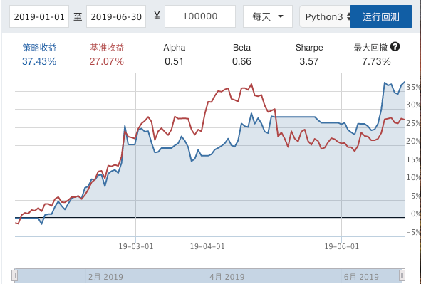
执行效果:
2、record函数——画图函数
调用record函数可用来描画额外的曲线。
参数:一个或多个key=value形式的参数,key为曲线名称,value为值。
在双均线策略中加入画图函数:
# 导入函数库
from jqdata import *

# 初始化函数,设定基准等等
def initialize(context):
    # 设定沪深300作为基准
    set_benchmark('000300.XSHG')
    # 开启动态复权模式(真实价格)
    set_option('use_real_price', True)
    # 股票类每笔交易时的手续费是:买入时佣金万分之三,卖出时佣金万分之三加千分之一印花税, 每笔交易佣金最低扣5块钱
    set_order_cost(OrderCost(close_tax=0.001, open_commission=0.0003, close_commission=0.0003, min_commission=5), type='stock')

    g.security = ["601318.XSHG"]
    g.p1 = 5      # 五日均线
    g.p2 = 10     # 十日均线


def handle_data(context, data):
    # 遍历股票
    for stock in g.security:
        df = attribute_history(stock, g.p2)
        # 十日均线的值
        ma10 = df['close'].mean()
        # 五日均线的值
        ma5 = df['close'][-5:].mean()

        if ma10 > ma5 and stock in context.portfolio.positions:   # 具有持仓
            # 死叉卖出
            order_target(stock, 0)
        if ma10 < ma5 and stock not in context.portfolio.positions:    # 不具有持仓
            # 金叉买入
            # order(stock, context.portfolio.available_cash)       # 能买多少买多少
            order(stock, context.portfolio.available_cash * 0.8)         # 可用资金的80%买入
    record(ma5=ma5, ma10=ma10)
执行显示如下:


 浙公网安备 33010602011771号