图像分割系列：OTSU算法

大津法（OTSU法）

介绍

大津法是由日本学者OTSU于1979年提出的一种像素级的图像分割方法，旨在利用阈值将原图像分成前景和背景两类，其思想在于最大化类间方差。当然也可以采用最小化类内方差和最大化类间方差。

原理

假定一幅灰度图像\(I(i,j)\)的灰度区间为\([0,L-1]\)，选择一个阈值thresh将图像的像素分为\(C_1\)和\(C_2\)两组。

\[\begin{eqnarray*} \left\{\begin{array}{l} C_1\quad I(i,j)\leq \text{thresh} \quad |C_1|=w_1,灰度均值m_1,方差\sigma_1^2\\ C_2\quad I(i,j)>\text{thresh} \quad |C_2|=w_2,灰度均值m_2,方差\sigma_2^2 \end{array} \right. \end{eqnarray*} \]

由此可以得到，以下几个数据。

• 图像总像素\(|I|=w_1+w_2\)，图像灰度均值为\(m=\frac{m_1w_1+m_2w_2}{w_1+w_2}\)。
• 类内离散度\(S_w=S_1+S_2\)，\(S_w=w_1\sigma_1^2+w_2\sigma_2^2\)。
• 类间离散度\(S_b=w_1(m_1-m)^2+w_2(m_2-m)^2=\frac{w_1w_2}{w_1+w_2}(m_1-m_2)^2\)

说明：网上还有一种版本采用概率的形式，如\(p_1=\frac{w_1}{w_1+w_2}\)，同样可以得到相同结果。另外，需要指出此处的类间离散度与Fisher线性判别分析中的定义是有所区别的，LDA采用类间离散度矩阵是\(S_b=(m_1-m_2)(m_1-m_2)^T\)。

分类的判别依据就是类间离散度越大越好，类内离散度越小越好。因此，\(S_b/S_w\)的值越大，则分割效果越好。可以采用遍历方式搜索整个灰度区间，找到最优thresh。这种分割方法也有一个明显的缺点，它没有考虑图像的几何结构，有时分割结果并不能令人满意。

实现

本文给出Python版本的实现方法，先获得图像像素的统计信息，然后遍历像素计算判别值，得到最优分割像素值。

def ThOTSU(img):
    A = img.flatten()
    A = np.sort(A)
    lst, uni_ind = np.unique(A,return_inverse=True)   
    del A
    num = np.diff(uni_ind) 
    count = []
    #统计不同像素的个数
    i = 1
    for x in num:
        if x==0:
            i = i+1
        else:     
            count.append(i)
            i = 1
    else:
        count.append(i)
    # 初始化均值，方差，类内离散度，类间离散度
    w1 = count[0]
    w2 = np.sum(count[1:])
    m1 = lst[0]
    m2 = (lst@count-w1*m1)/w2
    thresh = lst[0]
    sigma1 = 0
    sigma2 = (lst[1:]-m2)**2 @ count[1:] / (w2)
    Sw = w2*sigma2
    Sb = w1*w2/(w1+w2)*(m1-m2)**2
    score = Sb/Sw
    # 遍历像素区间寻找最优分割点
    for i in range(1,len(lst)-1):
        w1_new = w1 + count[i]
        w2_new = w2 - count[i]
        m1_new = (m1*w1 + lst[i]*count[i])/w1_new
        m2_new = (m2*w2 - lst[i]*count[i])/w2_new
        sigma1_new = (lst[:i]-m1_new)**2 @ count[:i] / (w1_new)
        sigma2_new = (lst[i:]-m2_new)**2 @ count[i:] / (w2_new)
        Sw = w1_new*sigma1_new + w2_new*sigma2_new
        Sb = w1_new*w2_new/(w1_new+w2_new)*(m1_new-m2_new)**2
        if Sb/Sw > score:
            score = Sb/Sw
            thresh = lst[i]
        w1, w2, m1, m2 = w1_new,w2_new,m1_new,m2_new
        sigma1, sigma2 = sigma1_new, sigma2_new
    return thresh

测试

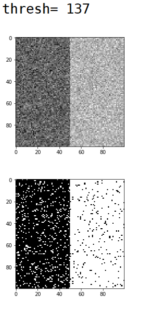
采用仿真，图片左半边像素采用均值为100方差为30的高斯分布，右半边采用均值为180方差为25的高斯分布，随机生成图像。

import numpy as np
import matplotlib.pyplot as plt
np.random.seed(1)
part1 = np.random.randn(100,50)*30+100
part1 = np.clip(part1,0,200).astype(np.uint8)
part2 = np.random.randn(100,50)*25+180
part2 = np.clip(part2,100,255).astype(np.uint8)
img = np.concatenate((part1,part2),axis=1)
plt.figure(1)
plt.imshow(img,'gray')

thresh = ThOTSU(img)
img2 = img>thresh
plt.figure(2)
plt.imshow(img2,'gray')

print("thresh=",ThOTSU(img))

得到仿真结果