Logistic回归之基于最优化方法的最佳回归系数确定

 

之前学习Java的时候，用过一个IDE叫做EditPlus,虽然他敲代码的高亮等体验度不及eclipse，但是打开软件特别快捷，现在也用他读python特别方便。

 

训练算法:：使用梯度上升找到最佳参数

之前看过吴恩达的视频的同学们，听得比较多的就是梯度下降算法，但是梯度上升算法和梯度下降算法本质是是一样的，只是梯度计算的时候加减号不一样罢了。

 

def loadDataSet():
    dataMat = []; labelMat = []
    fr = open('testSet.txt')
    for line in fr.readlines():
        lineArr = line.strip().split()
        dataMat.append([1.0, float(lineArr[0]), float(lineArr[1])])
        labelMat.append(int(lineArr[2]))
    return dataMat,labelMat

def sigmoid(inX):
    return 1.0/(1+exp(-inX))

def gradAscent(dataMatIn, classLabels):
    dataMatrix = mat(dataMatIn)             #convert to NumPy matrix
    labelMat = mat(classLabels).transpose() #convert to NumPy matrix
    m,n = shape(dataMatrix)
    alpha = 0.001
    maxCycles = 500
    weights = ones((n,1))
    for k in range(maxCycles):              #heavy on matrix operations
        h = sigmoid(dataMatrix*weights)     #matrix mult
        error = (labelMat - h)              #vector subtraction
        weights = weights + alpha * dataMatrix.transpose()* error #matrix mult
    return weights

第一个函数打开testSet。txt并逐行读取，每行前两个值分别是x1和x2，第三个值是对应的类别标签。为了方便计算，该函数还将x0的值设为1.0

第二个函数是sigmoid函数，x为0时，函数值为0.5，x增大时，函数值将不断增大逼近1。

第三个函数有两个参数，第一个是2维数组，每列代表不同的特征，每行代表每个训练样本。我们采用100个样本的简单数据集它包含两个特征x1,x2，再加上第0维特征x0,所以dataMatln里面存放的是100*3的矩阵。

 

 

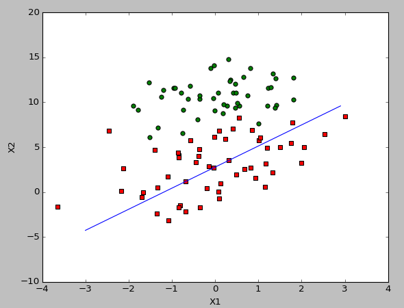
分析数据：画出决策边界

def plotBestFit(weights):
    import matplotlib.pyplot as plt
    dataMat,labelMat=loadDataSet()
    dataArr = array(dataMat)
    n = shape(dataArr)[0] 
    xcord1 = []; ycord1 = []
    xcord2 = []; ycord2 = []
    for i in range(n):
        if int(labelMat[i])== 1:
            xcord1.append(dataArr[i,1]); ycord1.append(dataArr[i,2])
        else:
            xcord2.append(dataArr[i,1]); ycord2.append(dataArr[i,2])
    fig = plt.figure()
    ax = fig.add_subplot(111)
    ax.scatter(xcord1, ycord1, s=30, c='red', marker='s')
    ax.scatter(xcord2, ycord2, s=30, c='green')
    x = arange(-3.0, 3.0, 0.1)
    y = (-weights[0]-weights[1]*x)/weights[2]
    ax.plot(x, y)
    plt.xlabel('X1'); plt.ylabel('X2');
    plt.show()

 

>>> from numpy import *
>>> reload(logRegres)
<module 'logRegres' from 'D:\Python27\logRegres.pyc'>
>>> weights=logRegres.gradAscent(dataArr,labelMat)
>>> logRegres.plotBestFit(weights.getA())

 

训练算法：随机梯度上升

梯度上升算法在每次更新回归系数时都需要遍历整个数据集。改进的方法是一次仅使用一个样本点来更新回归系数，该方法称为随机梯度上升算法。由于可以在样本到来时对分类器进行增量式更新，因而随机梯度上升算法是一个在线学习算法。与在线学习相对应，一次处理所有数据被称作是批处理。

def stocGradAscent0(dataMatrix, classLabels):
    m,n = shape(dataMatrix)
    alpha = 0.01
    weights = ones(n)   #initialize to all ones
    for i in range(m):
        h = sigmoid(sum(dataMatrix[i]*weights))
        error = classLabels[i] - h
        weights = weights + alpha * error * dataMatrix[i]
    return weights

 

>>> from numpy import *
>>> reload(logRegres)
<module 'logRegres' from 'D:\Python27\logRegres.pyc'>
>>> dataArr,labelMat=logRegres.loadDataSet()
>>> weights=logRegres.stocGradAscent0(array(dataArr),labelMat)
>>> logRegres.plotBestFit(weights)

 

 

改进的随机梯度上升算法

def stocGradAscent1(dataMatrix, classLabels, numIter=150):
    m,n = shape(dataMatrix)
    weights = ones(n)   #initialize to all ones
    for j in range(numIter):
        dataIndex = range(m)
        for i in range(m):
            alpha = 4/(1.0+j+i)+0.0001    #apha decreases with iteration, does not 
            randIndex = int(random.uniform(0,len(dataIndex)))#go to 0 because of the constant
            h = sigmoid(sum(dataMatrix[randIndex]*weights))
            error = classLabels[randIndex] - h
            weights = weights + alpha * error * dataMatrix[randIndex]
            del(dataIndex[randIndex])
    return weights

 增加了亮出代码来进行改进。一方面，alpha在每次迭代的时候都会调整，虽然alpha会随着迭代次数不断减小，但永远不会减小到0，因为存在一个常数项。

另一方面，通过随机选取样本来更新回归系数。

>>> dataArr,labelMat=logRegres.loadDataSet()
>>> weights=logRegres.stocGradAscent1(array(dataArr),labelMat)
>>> logRegres.plotBestFit(weights)

 

 

 从疝气病症预测病马的死亡率

def classifyVector(inX, weights):
    prob = sigmoid(sum(inX*weights))
    if prob > 0.5: return 1.0
    else: return 0.0

def colicTest():
    frTrain = open('horseColicTraining.txt'); frTest = open('horseColicTest.txt')
    trainingSet = []; trainingLabels = []
    for line in frTrain.readlines():
        currLine = line.strip().split('\t')
        lineArr =[]
        for i in range(21):
            lineArr.append(float(currLine[i]))
        trainingSet.append(lineArr)
        trainingLabels.append(float(currLine[21]))
    trainWeights = stocGradAscent1(array(trainingSet), trainingLabels, 1000)
    errorCount = 0; numTestVec = 0.0
    for line in frTest.readlines():
        numTestVec += 1.0
        currLine = line.strip().split('\t')
        lineArr =[]
        for i in range(21):
            lineArr.append(float(currLine[i]))
        if int(classifyVector(array(lineArr), trainWeights))!= int(currLine[21]):
            errorCount += 1
    errorRate = (float(errorCount)/numTestVec)
    print "the error rate of this test is: %f" % errorRate
    return errorRate

def multiTest():
    numTests = 10; errorSum=0.0
    for k in range(numTests):
        errorSum += colicTest()
    print "after %d iterations the average error rate is: %f" % (numTests, errorSum/float(numTests))

第一个函数，如果sigmoid值大于0.5函数返回1，否则返回0.

第二个函数，用于打开测试集和训练集，并对数据进行格式化处理的函数。

第三个函数，调用第二个函数10次并求结果的平均值。

                   .-' _..`.                  /  .'_.'.'                 | .' (.)`.                 ;'   ,_   `. .--.__________.'    ;  `.;-'|  ./               /|  |               / `..'`-._  _____, ..'     / | |     | |\ \    / /| |     | | \ \   / / | |     | |  \ \  /_/  |_|     |_|   \_\ |__\  |__\    |__\  |__\