机器学习项目实战----信用卡欺诈检测(二)
六、混淆矩阵:
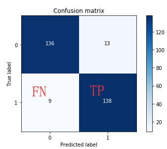
混淆矩阵是由一个坐标系组成的,有x轴以及y轴,在x轴里面有0和1,在y轴里面有0和1。x轴表达的是预测的值,y轴表达的是真实的值。可以对比真实值与预测值之间的差异,可以计算当前模型衡量的指标值。
这里精度的表示:(136+138)/(136+13+9+138)。之前有提到recall=TP/(TP+FN),在这里的表示具体如下:
下面定义绘制混淆矩阵的函数:
def plot_confusion_matrix(cm,
                          classes,
                          title='Confusion matrix',
                          cmap=plt.cm.Blues):
    # This function prints and plots the confusion matrix
    plt.imshow(cm, interpolation='nearest', cmap=cmap)
    plt.title(title)
    plt.colorbar()
    tick_marks = np.arange(len(classes))
    plt.xticks(tick_marks, classes, rotation=0)
    plt.yticks(tick_marks, classes)

    # cneter 改为 center
    thresh = cm.max() / 2
    for i, j in itertools.product(range(cm.shape[0]), range(cm.shape[1])):
        plt.text(j,
                 i,
                 cm[i, j],
                 horizontalalignment="center",
                 color="white" if cm[i, j] > thresh else "black")

    plt.tight_layout()
    plt.ylabel("True label")
    plt.xlabel("Predicted label")
下面根据上面得出的最好的那个C值,根据下采样数据集绘制出混淆矩阵。
import itertools

lr = LogisticRegression(C=best_c, penalty='l1', solver='liblinear')
lr.fit(X_train_undersample, y_train_undersample.values.ravel())
y_pred_undersample = lr.predict(X_test_undersample.values)

# Compute confusion matrix
cnf_matrix = confusion_matrix(y_test_undersample, y_pred_undersample)
np.set_printoptions(precision=2)

print("Recall metric in the testing dataset:",
      cnf_matrix[1, 1] / (cnf_matrix[1, 0] + cnf_matrix[1, 1]))

# Plot non-normalized confusion.matrix
class_names = [0, 1]
plt.figure()
plot_confusion_matrix(cnf_matrix,
                      classes=class_names,
                      title='Confusion matrix')
plt.show()
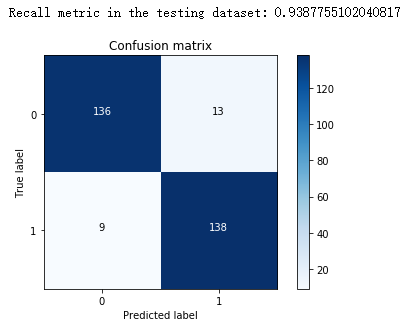
可以看出recall值达到93%,但是因为上面测试数据集采用的下采样数据集,数据利用率太低。
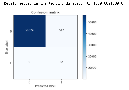
下面根据原始的划分的测试数据集来进行测试:
lr = LogisticRegression(C=best_c, penalty='l1', solver='liblinear')
lr.fit(X_train_undersample, y_train_undersample.values.ravel())
y_pred = lr.predict(X_test.values)

# Compute confusion matrix
cnf_matrix = confusion_matrix(y_test, y_pred)
np.set_printoptions(precision=2)

print("Recall metric in the testing dataset:",
      cnf_matrix[1, 1] / (cnf_matrix[1, 0] + cnf_matrix[1, 1]))

# Plot non-normalized confusion matrix
class_names = [0, 1]
plt.figure()
plot_confusion_matrix(cnf_matrix,
                      classes=class_names,
                      title="Confusion matrix")
plt.show()
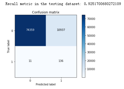
可以看到,这次测试的样本数据有八万多。达到的效果还行。这里误预测的值有一万多个,有点小多。
那下面如果我们直接拿原始数据集来进行建模,来看看在样本数据集分布不均衡的情况recall值的情况。
best_c = printing_Kfold_scores(X_train, y_train)
-------------------------------------------
C parameter: 0.01
-------------------------------------------

Iteration  0 : recall score =  0.4925373134328358
Iteration  1 : recall score =  0.6027397260273972
Iteration  2 : recall score =  0.6833333333333333
Iteration  3 : recall score =  0.5692307692307692
Iteration  4 : recall score =  0.45

Mean recall score  0.5595682284048672

-------------------------------------------
C parameter: 0.1
-------------------------------------------

Iteration  0 : recall score =  0.5671641791044776
Iteration  1 : recall score =  0.6164383561643836
Iteration  2 : recall score =  0.6833333333333333
Iteration  3 : recall score =  0.5846153846153846
Iteration  4 : recall score =  0.525

Mean recall score  0.5953102506435158

-------------------------------------------
C parameter: 1
-------------------------------------------

Iteration  0 : recall score =  0.5522388059701493
Iteration  1 : recall score =  0.6164383561643836
Iteration  2 : recall score =  0.7166666666666667
Iteration  3 : recall score =  0.6153846153846154
Iteration  4 : recall score =  0.5625

Mean recall score  0.612645688837163

-------------------------------------------
C parameter: 10
-------------------------------------------

Iteration  0 : recall score =  0.5522388059701493
Iteration  1 : recall score =  0.6164383561643836
Iteration  2 : recall score =  0.7333333333333333
Iteration  3 : recall score =  0.6153846153846154
Iteration  4 : recall score =  0.575

Mean recall score  0.6184790221704963

-------------------------------------------
C parameter: 100
-------------------------------------------

Iteration  0 : recall score =  0.5522388059701493
Iteration  1 : recall score =  0.6164383561643836
Iteration  2 : recall score =  0.7333333333333333
Iteration  3 : recall score =  0.6153846153846154
Iteration  4 : recall score =  0.575

Mean recall score  0.6184790221704963

*********************************************************************************
Best model to choose from cross validation is with C parameter 10.0
*********************************************************************************
可以看出,recall值基本在60%左右。
绘制出混淆矩阵看看:
lr = LogisticRegression(C=best_c, penalty='l1', solver='liblinear')
lr.fit(X_train, y_train.values.ravel())
# 注意这里不是x_pred_undersample 而是y_pred_undersample
y_pred_undersample = lr.predict(X_test.values)

# Compute confusion matrix
cnf_matrix = confusion_matrix(y_test, y_pred_undersample)
np.set_printoptions(precision=2)

print("Recall metric in the testing dataset",
      cnf_matrix[1, 1] / (cnf_matrix[1, 0] + cnf_matrix[1, 1]))

# Plot non-normalized confusion matrix
class_names = [0, 1]
plt.figure()
plot_confusion_matrix(cnf_matrix,
                      classes=class_names,
                      title='Confusison matrix')
plt.show()

可以看出,在样本数据分布不均衡的情况下,直接进行建立模型,结果并不太好。
在以前学习的逻辑回归模型中,默认是根据0.5来对结果进行分类。那我们可以作出猜想,可不可以通过改变这个阈值来确定到底哪个阈值对模型的最终结果更好呢?
lr = LogisticRegression(C=0.01, penalty='l1', solver='liblinear')
lr.fit(X_train_undersample, y_train_undersample.values.ravel())
y_pred_undersample_proba = lr.predict_proba(X_test_undersample.values) # 返回预测的概率值

thresholds = [0.1, 0.2, 0.3, 0.4, 0.5, 0.6, 0.7, 0.8, 0.9] # 阈值列表
plt.figure(figsize=(10, 10))

j = 1
for i in thresholds:
    y_test_predictions_high_recall = y_pred_undersample_proba[:, 1] > i
    plt.subplot(3, 3, j)
    j += 1

    # Compute confusion matrix
    cnf_matrix = confusion_matrix(y_test_undersample,
                                  y_test_predictions_high_recall)
    np.set_printoptions(precision=2)

    print("Recall metric in the testing dataset:",
          cnf_matrix[1, 1] / (cnf_matrix[1, 0] + cnf_matrix[1, 1]))

    # Plot non-normalized confusion matrix
    class_names = [0, 1]
    plot_confusion_matrix(cnf_matrix,
                          classes=class_names,
                          title='Threshold >= %s' % i)
Recall metric in the testing dataset: 1.0
Recall metric in the testing dataset: 1.0
Recall metric in the testing dataset: 1.0
Recall metric in the testing dataset: 0.9795918367346939
Recall metric in the testing dataset: 0.9387755102040817
Recall metric in the testing dataset: 0.891156462585034
Recall metric in the testing dataset: 0.8367346938775511
Recall metric in the testing dataset: 0.7687074829931972
Recall metric in the testing dataset: 0.5850340136054422

图上可以看出,不同的阈值,混淆矩阵是长什么样子的。根据精度、recall值和误预测的值来综合考虑,可以看出阈值在0.5和0.6模型的效果不错。
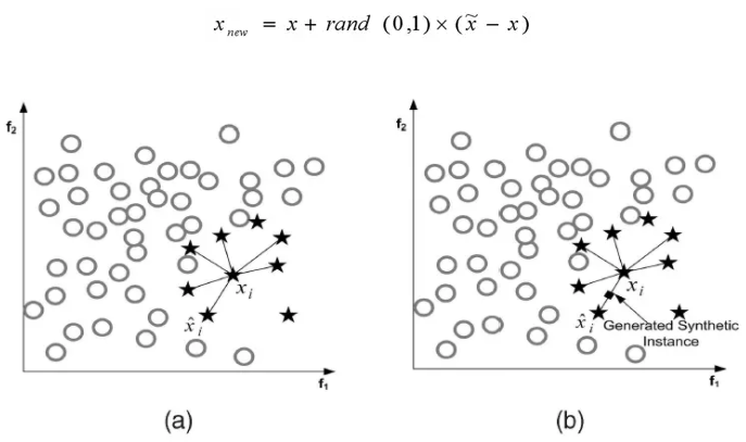
七、过采样操作
过采样操作(SMOTE算法):
(1)对于少数类中每一个样本x,以欧氏距离为标准计算它到少数类样本集中所有样本的距离,得到其k近邻。
(2)根据样本不平衡比例设置一个采样比例以确定采样倍率N,对于每一个少数类样本x,从其k近邻中随机选择若干个样本,假设选择的近邻为xn。
(3)对于每一个随机选出的近邻xn,分别与原样本按照如下的公式构建新的样本。
导入相关的Python库
import pandas as pd
from imblearn.over_sampling import SMOTE  # pip install imblearn
from sklearn.ensemble import RandomForestClassifier
from sklearn.metrics import confusion_matrix
from sklearn.model_selection import train_test_split
得到特征和标签数据
credit_cards = pd.read_csv('creditcard.csv')

columns = credit_cards.columns
# The labels are in the last column ('Class'). Simply remove it to obtain features columns
features_columns = columns.delete(len(columns) - 1)

features = credit_cards[features_columns]
labels = credit_cards['Class']
划分训练集测试集
features_train, features_test, labels_train, labels_test = train_test_split(
    features, labels, test_size=0.2, random_state=0)
根据SMOTE算法得到过采样数据集
oversampler = SMOTE(random_state=0)
os_features,os_labels = oversampler.fit_sample(features_train,labels_train) # OS  oversampler
可以看看过采样数据集大小
len(os_labels[os_labels==1])
227454
下面根据过采样数据集来进行交叉验证及逻辑回归模型建立
os_features = pd.DataFrame(os_features)
os_labels = pd.DataFrame(os_labels)
best_c = printing_Kfold_scores(os_features, os_labels)
-------------------------------------------
C parameter: 0.01
-------------------------------------------

Iteration  0 : recall score =  0.8903225806451613
Iteration  1 : recall score =  0.8947368421052632
Iteration  2 : recall score =  0.9687728228394379
Iteration  3 : recall score =  0.9578813158791396
Iteration  4 : recall score =  0.958167089831943

Mean recall score  0.933976130260189

-------------------------------------------
C parameter: 0.1
-------------------------------------------

Iteration  0 : recall score =  0.8903225806451613
Iteration  1 : recall score =  0.8947368421052632
Iteration  2 : recall score =  0.9703884032311608
Iteration  3 : recall score =  0.9593981160901727
Iteration  4 : recall score =  0.9605082379837548

Mean recall score  0.9350708360111024

-------------------------------------------
C parameter: 1
-------------------------------------------

Iteration  0 : recall score =  0.8903225806451613
Iteration  1 : recall score =  0.8947368421052632
Iteration  2 : recall score =  0.9704105344694036
Iteration  3 : recall score =  0.9585847594552709
Iteration  4 : recall score =  0.9595410030665743

Mean recall score  0.9347191439483347

-------------------------------------------
C parameter: 10
-------------------------------------------

Iteration  0 : recall score =  0.8903225806451613
Iteration  1 : recall score =  0.8947368421052632
Iteration  2 : recall score =  0.9705433218988603
Iteration  3 : recall score =  0.9601894901133203
Iteration  4 : recall score =  0.9604862553720007

Mean recall score  0.9352556980269211

-------------------------------------------
C parameter: 100
-------------------------------------------

Iteration  0 : recall score =  0.8903225806451613
Iteration  1 : recall score =  0.8947368421052632
Iteration  2 : recall score =  0.9703220095164324
Iteration  3 : recall score =  0.9604093162308613
Iteration  4 : recall score =  0.9607170727954188

Mean recall score  0.9353015642586275

*********************************************************************************
Best model to choose from cross validation is with C parameter 100.0
*********************************************************************************
再来看看混淆矩阵
lr = LogisticRegression(C = best_c, penalty = 'l1', solver='liblinear')
lr.fit(os_features,os_labels.values.ravel())
y_pred = lr.predict(features_test.values)

# Compute confusion matrix
cnf_matrix = confusion_matrix(labels_test,y_pred)
np.set_printoptions(precision=2)

print("Recall metric in the testing dataset: ", cnf_matrix[1,1]/(cnf_matrix[1,0]+cnf_matrix[1,1]))

# Plot non-normalized confusion matrix
class_names = [0,1]
plt.figure()
plot_confusion_matrix(cnf_matrix
                      , classes=class_names
                      , title='Confusion matrix')
plt.show()
经过前面的学习,综合考虑精度,recall值和误预测的值,发现过采样的效果比下采样的效果要好一点。
八、总结:
对于样本不均衡数据,要利用越多的数据越好。下采样误预测值很高,这是模型本身自带的一个问题,因为0和1一样少,模型会认为原始数据0和1的数据一样少,导致误预测值偏高。在这次的案例中,过采样的结果偏好一些,虽然recall偏低了一点,但是整体的效果还是不错的。
流程:
(1)首先要观察数据,当前数据是否分布均衡,不均衡的情况下就要想一些方法。(这次的数据是比较纯净的,就不需要做其他一些预处理的操作,直接原封不动的拿出来就可以了。很多情况下,不见得可以直接拿到特征数据。)
(2)让数据进行标准化,让数据的浮动比较小一些,然后再进行数据的选择。
(3)混淆矩阵以及模型的评估标准,然后通过交叉验证的方式来进行参数的选择。
(4)通过阈值与预测值进行比较,然后得到最终的一个预测结果。不同的阈值会使结果发生很大的变化。
(5)SMOTE算法。
通过对信用卡欺诈检测这个案例了解了机器学习中样本数据分布不均衡的解决方案、交叉验证、正则化惩罚、混淆矩阵和模型的评估方法等等。
本文来自博客园,作者:|旧市拾荒|,转载请注明原文链接:https://www.cnblogs.com/xiaoyh/p/11209909.html

 浙公网安备 33010602011771号