

机器学习之使用Python完成逻辑回归
一、任务基础
我们将建立一个逻辑回归模型来预测一个学生是否被大学录取。假设你是一个大学系的管理员,你想根据两次考试的结果来决定每个申请人的录取机会。你有以前的申请人的历史数据,你可以用它作为逻辑回归的训练集。对于每一个培训例子,你有两个考试的申请人的分数和录取决定。为了做到这一点,我们将建立一个分类模型,根据考试成绩估计入学概率。
数据集链接为:链接:https://pan.baidu.com/s/1H3T3RfyT3toKbFrqO2z8ug,提取码:jku5
首先导入需要使用到的Python库:
# 数据分析三个必备的python库
import numpy as np
import pandas as pd
import matplotlib.pyplot as plt
%matplotlib inline
读取数据然后查看数据:
import os

path = "data" + os.sep + "LogiReg_data.txt"
# header=None 表示没有列标签 第三列表示考生是否被录取 Exam 1 Exam 2  表示两个特征
pdData = pd.read_csv(path, header=None, names=['Exam 1', 'Exam 2', 'Admitted'])
pdData.head()
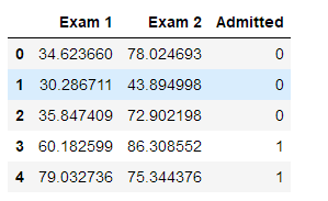
查看数据维度:
pdData.shape
(100, 3)
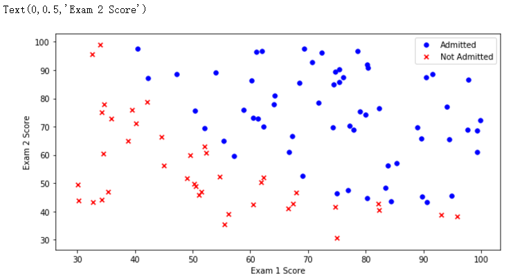
根据是否录取为标准,查看数据集的分布
# pdData 是二维数组
positive = pdData[pdData['Admitted'] == 1]
negative = pdData[pdData['Admitted'] == 0]

fig, ax = plt.subplots(figsize=(10, 5))
# 绘制散点图
ax.scatter(positive['Exam 1'],
           positive['Exam 2'],
           s=30,
           c='b',
           marker='o',
           label='Admitted')
ax.scatter(negative['Exam 1'],
           negative['Exam 2'],
           s=30,
           c='r',
           marker='x',
           label='Not Admitted')
ax.legend()  # 添加图例
ax.set_xlabel('Exam 1 Score')
ax.set_ylabel('Exam 2 Score')
二、定义函数模块
接下来按照模块化编程:
θ0表示第一个考试成绩权重,θ1表示第二个考试成绩权重,θ2表示偏置项

首先,定义Sigmoid函数
def sigmoid(z):
    return 1 / (1 + np.exp(-z))
查看Sigmoid函数图像:
# sigmoid函数图像
nums = np.arange(-10, 10, step=1)
fig, ax = plt.subplots(figsize=(10, 5))
ax.plot(nums, sigmoid(nums), 'r')
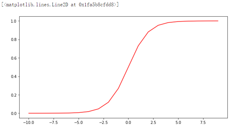
根据上图我们可以看到,这个函数的值域是0到1。当x趋近于负无穷时,y趋近于0,当x趋近于正无穷时,y趋近于1。并且当x等0时,y等于0.5。
返回预测结果值:
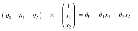
def model(X, theta):
    return sigmoid(np.dot(X, theta.T)) # 矩阵乘法
在第一列的前面在加上数据全为1的一列,为了方便上面的矩阵进行运算。
# pdData.drop('Ones', 1, inplace=True)  # 删除添加的Ones列
pdData.insert(0, 'Ones', 1)

orig_data = pdData.as_matrix()
# print(orig_data.shape)
cols = orig_data.shape[1]
X = orig_data[:, 0:cols - 1]
y = orig_data[:, cols - 1:cols]

# 三个θ参数,用零占位
theta = np.zeros([1, 3])
查看X五个样本数据
X[:5]

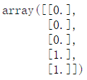
查看y五个样本数据
y[:5]
查看theta参数
theta
![]()
查看X,y,theta的维度
X.shape, y.shape, theta.shape
((100, 3), (100, 1), (1, 3))
根据以上,我们可以检查到前面都是没有问题的。使用Notebook开发就是这个好处,可以边做边检查。
根据参数计算损失:
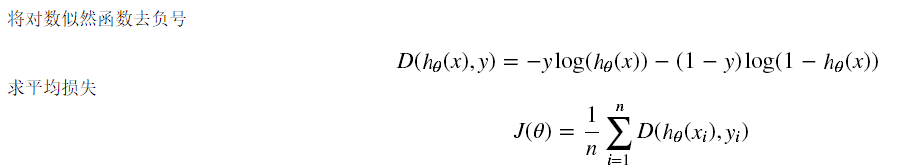
def cost(X, y, theta):
    left = np.multiply(-y, np.log(model(X, theta)))
    right = np.multiply(1 - y, np.log(1 - model(X, theta)))
    # print(left.shape)
    # print("===========================")
    # print(right.shape)
    return np.sum(left - right) / len(X)
计算cost值,检查cost函数是否正确
cost(X, y, theta)
0.6931471805599453
计算每个参数的梯度方向:
def gradient(X, y, theta):
    grad = np.zeros(theta.shape) # 一共三个参数  所以计算三个参数的梯度
    error = (model(X, theta) - y).ravel() # ravel展平数组
    for j in range(len(theta.ravel())):
        term = np.multiply(error, X[:, j])
        grad[0, j] = np.sum(term) / len(X) # grad[0, 0] grad[0, 1] grad[0, 2]
    return grad
比较3种不同梯度下降方法:
(1)批量梯度下降
(2)随机梯度下降
(3)小批量梯度下降
STOP_ITER = 0 # 按照迭代次数停止
STOP_COST = 1 # 按照损失值停止,两次迭代损失值很小则停止
STOP_GRAD = 2 # 根据梯度停止,梯度变化很小则停止


# threshold 阈值
def stopCriterion(type, value, threshold):
    # 设定三种不同的停止策略
    if type == STOP_ITER:
        return value > threshold
    elif type == STOP_COST:
        return abs(value[-1] - value[-2]) < threshold
    elif type == STOP_GRAD:
        return np.linalg.norm(value) < threshold
打乱数据,防止有规律数据
import numpy.random

# 打乱数据
def shuffleData(data):
    np.random.shuffle(data)
    cols = data.shape[1]
    X = data[:, 0:cols - 1]
    y = data[:, cols - 1:]
    return X, y
进行参数更新
import time

# 梯度下降求解  batchSize取1代表随机梯度下降,取总样本数代表梯度下降,取1~总样本数之间代表miniBatch梯度下降
def descent(data, theta, batchSize, stopType, thresh, alpha):
    init_time = time.time() # 初始时间  thresh:阈值,alpha:学习率
    i = 0 # 迭代次数
    k = 0 # batch
    X, y = shuffleData(data)
    grad = np.zeros(theta.shape) # 计算的梯度
    costs = [cost(X, y, theta)] #损失值

    while True:
        grad = gradient(X[k:k + batchSize], y[k:k + batchSize], theta)
        k += batchSize # 取batch数量个数据 n可能代表0
        if k >= n:
            k = 0
            X, y = shuffleData(data) # 重新打乱数据
        theta = theta - alpha * grad # 参数更新
        costs.append(cost(X, y, theta)) # 计算新的损失
        i += 1

        if stopType == STOP_ITER:
            value = i
        elif stopType == STOP_COST:
            value = costs
        elif stopType == STOP_GRAD:
            value = grad
        if stopCriterion(stopType, value, thresh):
            break
    return theta, i - 1, costs, grad, time.time() - init_time
进行结果的图像展示的展示
def runExpe(data, theta, batchSize, stopType, thresh, alpha):
    theta, iter, costs, grad, dur = descent(data, theta, batchSize, stopType,
                                            thresh, alpha)
    name = "Original" if (data[:, 1 > 2]).sum() > 1 else "Scaled"
    name += " data - learning rate:{} - ".format(alpha)
    if batchSize == n:
        strDescType = "Gradient"
    elif batchSize == 1:
        strDescType = "Stochastic"
    else:
        strDescType = "Mini-batch ({})".format(batchSize)
    name += strDescType + " descent - Stop: "
    if stopType == STOP_ITER:
        strStop = "{} iterations".format(thresh)
    elif stopType == STOP_COST:
        strStop = "costs change < {}".format(thresh)
    else:
        strStop = "gradient norm < {}".format(thresh)
    name += strStop
    print(
        "***{}\nTheta:{} - Iter:{} - Last cost: {:03.2f} - Duration:{:03.2f}s".
        format(name, theta, iter, costs[-1], dur))
    fig, ax = plt.subplots(figsize=(10, 5))
    ax.plot(np.arange(len(costs)), costs, 'r')
    ax.set_xlabel('Iterations')
    ax.set_ylabel('Cost')
    ax.set_title(name.upper() + ' - Error vs. Iteration')
    return theta
三、实验结果对比
下面对比三种停止策略对结果的影响
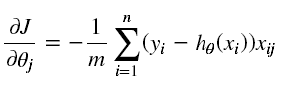
根据迭代次数停止,设定阈值5000次,也就是说迭代次数超过5000即停止迭代
n = 100 # 选择所有样本进行梯度下降
runExpe(orig_data, theta, n, STOP_ITER, thresh=5000, alpha=0.000001)
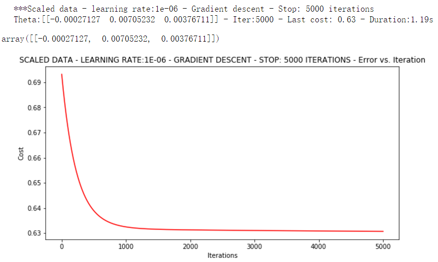
上面迭代了5000次,看起来似乎目标函数已经成功收敛。上面消耗一秒多的时间,看起来似乎不太行,损失值0.63。下面根据损失值停止,设定阈值1E-6,也就是两次损失值之差不能超过1E-6,差不多需要500000次迭代
runExpe(orig_data, theta, n, STOP_COST, thresh=0.0000001, alpha=0.001)
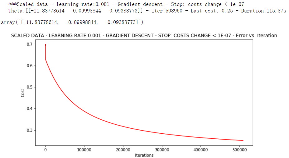
根据图片标题我们可以看到差不多迭代50万次才达到我们定义的阈值,而此时收敛的效果更好。损失值只有0.25,消耗的时间达到100多秒。下面根据梯度变化停止,设定阈值0.05,表示梯度相差0.05即停止迭代。
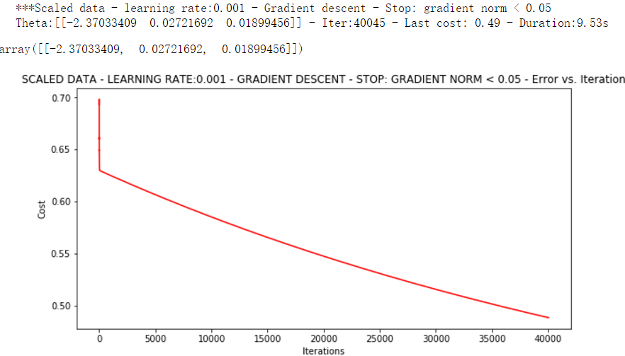
runExpe(orig_data, theta, n, STOP_GRAD, thresh=0.05, alpha=0.001)
下面这三种对比不同的梯度下降方法
下面1表示每次1次迭代只拿一个样本,batchSize取1代表随机梯度下降,取总样本数代表梯度下降,取1~总样本数之间代表miniBatch梯度下降
runExpe(orig_data, theta, 1, STOP_ITER, thresh=5000, alpha=0.001)
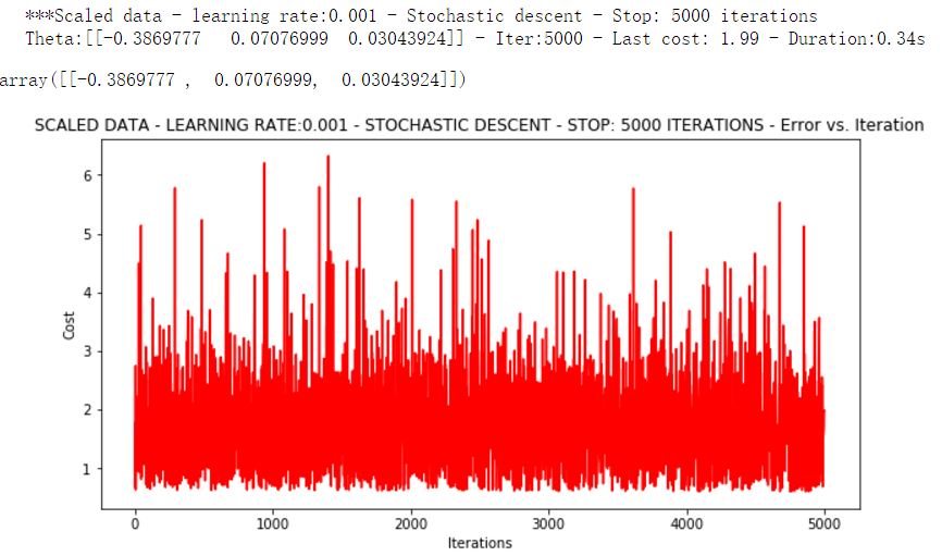
有点爆炸。。。很不稳定,下面把迭代次数调高点,学习率调低点
runExpe(orig_data, theta, 1, STOP_ITER, thresh=15000, alpha=0.000002)
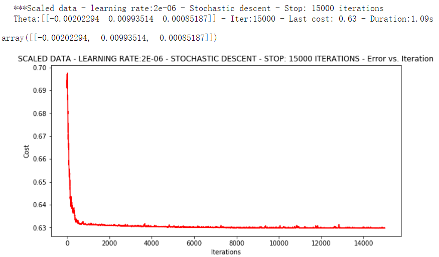
可以看出这次结果,速度快,但稳定性差,需要很小的学习率
下面进行Mini-batch descent,一次迭代拿16个样本。
runExpe(orig_data, theta, 16, STOP_ITER, thresh=15000, alpha=0.001)
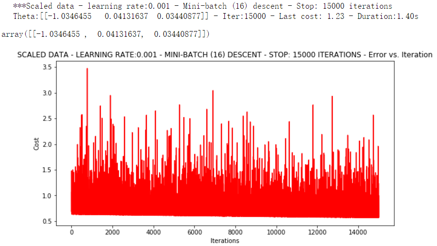
浮动仍然比较大,我们来尝试下对数据进行标准化:将数据按其属性(按列进行)减去其均值,然后除以其方差。最后得到的结果是,对每个属性/每列来说所有数据都聚集在0附近,方差值为1
from sklearn import preprocessing as pp

scaled_data = orig_data.copy()
scaled_data[:, 1:3] = pp.scale(orig_data[:, 1:3])

runExpe(scaled_data, theta, n, STOP_ITER, thresh=5000, alpha=0.001)
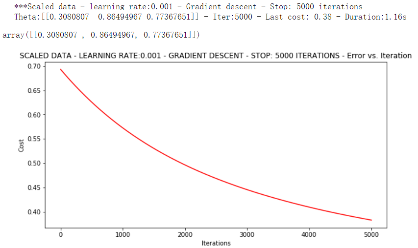
它好多了!原始数据,只能5000次迭代损失值达到0.61,而我们得到了0.38在这里! 所以对数据做预处理是非常重要的
runExpe(scaled_data, theta, n, STOP_GRAD, thresh=0.02, alpha=0.001)
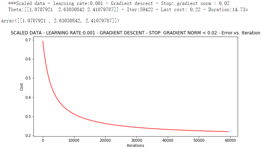
更多的迭代次数会使得损失下降的更多!
theta = runExpe(scaled_data, theta, 1, STOP_GRAD, thresh=0.002/5, alpha=0.001)
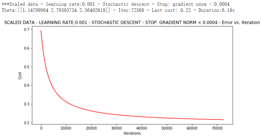
随机梯度下降更快,但是我们需要迭代的次数也需要更多,所以还是用batch的比较合适!!!
runExpe(scaled_data, theta, 16, STOP_GRAD, thresh=0.002*2, alpha=0.001)

这次时间只花了0.16秒,损失值只有0.22,迭代次数也只有一千多次,得到的结果不错。所以说当我们进行数据梯度下降的时候,首先对数据进行预处理,然后再进行各种的尝试,在这里的话Mini-batch是比较好的,无论是从时间还是结果来看。
预测函数
def predict(X, theta):
    return [1 if x >= 0.5 else 0 for x in model(X, theta)]
计算准确率
scaled_X = scaled_data[:, :3]
y = scaled_data[:, 3]
predictions = predict(scaled_X, theta)
correct = [
    1 if ((a == 1 and b == 1) or (a == 0 and b == 0)) else 0
    for (a, b) in zip(predictions, y)
]
accuracy = (sum(map(int, correct)) % len(correct))
print('accuracy = {0}'.format(accuracy))
最终得到准确率89%。
accuracy = 89%
总结:首先拿到数据集看下数据长什么样子,然后再给数据增加了一列全是1的数据,然后再对每个模块函数的编写,最后对比各种策略下的实验结果,最终得出最佳结果。
本文来自博客园,作者:|旧市拾荒|,转载请注明原文链接:https://www.cnblogs.com/xiaoyh/p/11158850.html

 浙公网安备 33010602011771号