李宏毅机器学习作业2！！！判断年收入。

这次作业依然是直接看的答案。数据处理这一步对我来说依然是过于困难。而且这次给的文件格式也不是传统的csv，而且说实话我也不知道是什么文件。用记事本打开格式也很乱，ggsimida。

开始开始。

import numpy as np

np.random.seed(0)
X_train_fpath = 'work/data/X_train'
Y_train_fpath = 'work/data/Y_train'
X_test_fpath = 'work/data/X_test'
output_fpath = 'work/output_{}.csv'

# Parse csv files to numpy array
with open(X_train_fpath) as f:        #为了更好关闭文件采用的写法，用来读文件，f指向X_TRAIN。open中的MODE不写，表示只读。
    next(f)                           #next用来迭代，每次向后读一行。这里用来跳过文件的第一行。
    X_train = np.array([line.strip('\n').split(',')[1:] for line in f], dtype = float)   #.strip用来移除字符串首尾指定的字符,split用来以逗号分割句子，
# 得到的结果相当于一个数组，所以后面可以用[1:]来表示下标1及后面的所有元素。for line in f是列表推导式的用法。对于f中的每个LINE都进行前面的操作。
with open(Y_train_fpath) as f:
    next(f)
    Y_train = np.array([line.strip('\n').split(',')[1] for line in f], dtype = float)
with open(X_test_fpath) as f:
    next(f)
    X_test = np.array([line.strip('\n').split(',')[1:] for line in f], dtype = float)

没啥好说的，直接一个文件的导入。 值得注意的是这次需要解压开文件，而上次第一次作业并没有解压。真是神奇啊！。其实从这里我们可以看到文件的结构。应该是跟给的EXCAL表格差不多的。

对 就是这样，第一行全是表项，通过next跳过。

def _normalize(X, train = True, specified_column = None, X_mean = None, X_std = None):
    # This function normalizes specific columns of X.
    # The mean and standard variance of training data will be reused when processing testing data.
    #
    # Arguments:
    #     X: data to be processed
    #     train: 'True' when processing training data, 'False' for testing data
    #     specific_column: indexes of the columns that will be normalized. If 'None', all columns
    #         will be normalized.
    #     X_mean: mean value of training data, used when train = 'False'
    #     X_std: standard deviation of training data, used when train = 'False'
    # Outputs:
    #     X: normalized data
    #     X_mean: computed mean value of training data
    #     X_std: computed standard deviation of training data

    if specified_column == None:
        specified_column = np.arange(X.shape[1])#.shape()中 若参数是空，输出行列。若是0则输出行数。若为1输出列数#np.arrange（x） 用来输出0到x的一个列表。返回列表
    if train:
        # print('1',specified_column.shape)
        # print('1',X.shape)
        X_mean = np.mean(X[:, specified_column], 0).reshape(1, -1)
        # X_mean = np.mean(X ,0)
        # print('1',X_mean.shape)
        # X_mean=X_mean.reshape(1, -1)
        # print('2',X_mean.shape)
        X_std  = np.std(X[:, specified_column], 0).reshape(1, -1)

    X[:,specified_column] = (X[:, specified_column] - X_mean) / (X_std + 1e-8)  #将列归一化，中心化和标准化处理。

    return X, X_mean, X_std

这一片是正则化函数，实现的是如果是train数据，就求TRAIN的均值方差来正则化，如果是test就用train的均值方差正则化。请注意为了防止方差为0，这里总会加一个极小量。

def _train_dev_split(X, Y, dev_ratio = 0.25):
    # This function spilts data into training set and development set.
    train_size = int(len(X) * (1 - dev_ratio))
    return X[:train_size], Y[:train_size], X[train_size:], Y[train_size:]#前面的列隐含了，截取的行。

老任务了，将训练的样本分为两部分，一部分用来训练，一部分用来测试 这里截取了90%的数据来训练。

def _shuffle(X, Y):  #洗牌，排序
    # This function shuffles two equal-length list/array, X and Y, together.
    randomize = np.arange(len(X))
    np.random.shuffle(randomize)
    return (X[randomize], Y[randomize])    #作用是将行重新打乱。

  这个函数能将一个矩阵的行乱序。为的是每次循环时用不一样的数据。

def _sigmoid(z):             #不谈了吧
    # Sigmoid function can be used to calculate probability.
    # To avoid overflow, minimum/maximum output value is set.
    return np.clip(1 / (1.0 + np.exp(-z)), 1e-8, 1 - (1e-8))#np.clip(a,min,max),作用是将所有输出的a都限制在min和max之间。

这个就不说了吧！

def _f(X, w, b):
    # This is the logistic regression function, parameterized by w and b
    #
    # Arguements:
    #     X: input data, shape = [batch_size, data_dimension]
    #     w: weight vector, shape = [data_dimension, ]
    #     b: bias, scalar
    # Output:
    #     predicted probability of each row of X being positively labeled, shape = [batch_size, ]
    return _sigmoid(np.matmul(X, w) + b)#二维乘法。

这个很重要，其实求出来就是那个要的概率，发现没？

def _predict(X, w, b):
    # This function returns a truth value prediction for each row of X
    # by rounding the result of logistic regression function.
    return np.round(_f(X, w, b)).astype(np.int)# 这里是取整，所以为神马要取整呢？

 

我开始不知道为啥要取整，后面想想 这是判断题嘛，只有错号和对号，所以落在我的半区就是我的人。取整就完事了。

def _accuracy(Y_pred, Y_label):
    # This function calculates prediction accuracy
    acc = 1 - np.mean(np.abs(Y_pred - Y_label))
    return acc   

这里输入标签和结果，会得到精确度。因为Y_p和Y_l都是0或者1 所以他们的绝对值就是不对的数量。求平均就是错误率。1减就是精准度。

def _cross_entropy_loss(y_pred, Y_label):
    # This function computes the cross entropy.
    #
    # Arguements:
    #     y_pred: probabilistic predictions, float vector
    #     Y_label: ground truth labels, bool vector
    # Output:
    #     cross entropy, scalar
    cross_entropy = -np.dot(Y_label, np.log(y_pred)) - np.dot((1 - Y_label), np.log(1 - y_pred))
    return cross_entropy

这里计算交叉熵，好像 似乎交叉熵对于优化的作用不大的样子。就是算算看看？

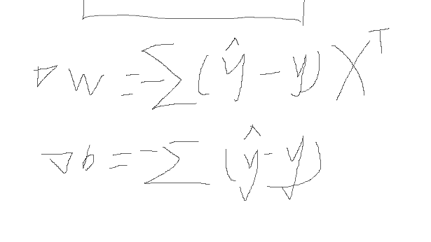
def _gradient(X, Y_label, w, b):
    # This function computes the gradient of cross entropy loss with respect to weight w and bias b.
    y_pred = _f(X, w, b)
    pred_error = Y_label - y_pred
    w_grad = -np.sum(pred_error * X.T, 1)  #axis=1 表示对行进行求和。
    b_grad = -np.sum(pred_error)
    return w_grad, b_grad
# Zero initialization for weights ans bias

 

下面开始学习。

1 数据正则化。训练集测试集都要正则。

# Normalize training and testing data
X_train, X_mean, X_std = _normalize(X_train, train = True)
X_test, _, _= _normalize(X_test, train = False, specified_column = None, X_mean = X_mean, X_std = X_std)
#测试集标准化时使用的是训练集的均值和标准差。 这里两个下划线用来承接返回的值，但没有用，所以用下划线。

# Split data into training set and development set
dev_ratio = 0.1
X_train, Y_train, X_dev, Y_dev = _train_dev_split(X_train, Y_train, dev_ratio = dev_ratio)

train_size = X_train.shape[0]
dev_size = X_dev.shape[0]
test_size = X_test.shape[0]
data_dim = X_train.shape[1]
print('Size of training set: {}'.format(train_size))
print('Size of development set: {}'.format(dev_size))
print('Size of testing set: {}'.format(test_size))
print('Dimension of data: {}'.format(data_dim))

# Zero initialization for weights ans bias
w = np.zeros((data_dim,))
b = np.zeros((1,))

# Some parameters for training
max_iter = 10
batch_size = 8
learning_rate = 0.2  #所以说 学习速度究竟如何设置呢？？？
开始啦开始啦 开始学习啦

# Keep the loss and accuracy at every iteration for plotting
train_loss = []
dev_loss = []
train_acc = []
dev_acc = []

# Iterative training
for epoch in range(max_iter):
    # Random shuffle at the begging of each epoch
    X_train, Y_train = _shuffle(X_train, Y_train)#打乱数据

    # Mini-batch training
    for idx in range(int(np.floor(train_size / batch_size))):#每次学八个数据。
        X = X_train[idx*batch_size:(idx+1)*batch_size]
        Y = Y_train[idx*batch_size:(idx+1)*batch_size]

        # Compute the gradient
        w_grad, b_grad = _gradient(X, Y, w, b)

        # gradient descent update
        # learning rate decay with time
        w = w - learning_rate/np.sqrt(step) * w_grad
        b = b - learning_rate/np.sqrt(step) * b_grad  #step越大，即越到后期，w改变的越少

        step = step + 1
到这里 完成一轮的计算，但是还要后面的记录。
    # Compute loss and accuracy of training set and development set
    y_train_pred = _f(X_train, w, b)
    # print('1',y_train_pred)
    Y_train_pred = np.round(y_train_pred)  #round无参数，四舍五入至最近的整数。
    # print('2',y_train_pred)
    # print(_accuracy(Y_train_pred, Y_train))
    train_acc.append(_accuracy(Y_train_pred, Y_train)) #append在矩阵后面附加值,这里形成一行。
    train_loss.append(_cross_entropy_loss(y_train_pred, Y_train) / train_size)

    y_dev_pred = _f(X_dev, w, b)
    Y_dev_pred = np.round(y_dev_pred)
    dev_acc.append(_accuracy(Y_dev_pred, Y_dev))
    dev_loss.append(_cross_entropy_loss(y_dev_pred, Y_dev) / dev_size)

这里就完了 下面是统计学
print('Training loss: {}'.format(train_loss[-1]))
print('Development loss: {}'.format(dev_loss[-1]))
print('Training accuracy: {}'.format(train_acc[-1]))
print('Development accuracy: {}'.format(dev_acc[-1])) #-1 应该是倒数第一个的意思吧 。最后一轮的值。

import matplotlib.pyplot as plt

# Loss curve
print(train_loss)
plt.plot(train_loss)#绘图
plt.plot(dev_loss)#绘图
plt.title('Loss')#标题
plt.legend(['train', 'dev'])#图例
plt.savefig('loss.png')#保存
plt.show()

# Accuracy curve
plt.plot(train_acc)
plt.plot(dev_acc)
plt.title('Accuracy')
plt.legend(['train', 'dev'])
plt.savefig('acc.png')
plt.show()

搞完训练搞测试
# Predict testing labels
predictions = _predict(X_test, w, b)
print(1111)
with open(output_fpath.format('logistic'), 'w') as f:
    f.write('id,label\n')
    for i, label in  enumerate(predictions):#enumerate是枚举函数，i就是下标，label就是pre中的元素。
        f.write('{},{}\n'.format(i, label))

# Print out the most significant weights
ind = np.argsort(np.abs(w))[::-1]#argsort返回的是从小到大排序的下标。后面是一个逆序。
with open(X_test_fpath) as f:
    content = f.readline().strip('\n').split(',')
print('content',content)
features = np.array(content)
for i in ind[0:10]:    #这个循环，就是让i去取ind中的每一个值。
    print(features[i], w[i])
找到最重要的那个权值，但说实话 我没看很懂.但应该是先排W，从小到大的索引出来，再逆序。找到前十名大的W。
下面就开始用解析解的方法了。

# Parse csv files to numpy array
with open(X_train_fpath) as f:
    next(f)
    X_train = np.array([line.strip('\n').split(',')[1:] for line in f], dtype = float)
with open(Y_train_fpath) as f:
    next(f)
    Y_train = np.array([line.strip('\n').split(',')[1] for line in f], dtype = float)
with open(X_test_fpath) as f:
    next(f)
    X_test = np.array([line.strip('\n').split(',')[1:] for line in f], dtype = float)

先导入文件。

# Normalize training and testing data
X_train, X_mean, X_std = _normalize(X_train, train = True)
X_test, _, _= _normalize(X_test, train = False, specified_column = None, X_mean = X_mean, X_std = X_std)

正则化

# Compute in-class mean
X_train_0 = np.array([x for x, y in zip(X_train, Y_train) if y == 0])     #zip打包函数，将两个对象的对应元素叠加打包成元组
X_train_1 = np.array([x for x, y in zip(X_train, Y_train) if y == 1])     #fx for x in z 会对z中每一个x都执行fx的操作。

将数据分为两组。label=1的label=0的分在不一样的组里。

mean_0 = np.mean(X_train_0, axis = 0)
mean_1 = np.mean(X_train_1, axis = 0)#   现在就将miu0 与 miu1分开了。

# Compute in-class covariance
cov_0 = np.zeros((data_dim, data_dim))
print('222',data_dim)
cov_1 = np.zeros((data_dim, data_dim))

for x in X_train_0:
    cov_0 += np.dot(np.transpose([x - mean_0]), [x - mean_0]) / X_train_0.shape[0]##其实这里等效于将数据矩阵的每一列都减去平均值后再进行X.TdotX的操作
for x in X_train_1:
    cov_1 += np.dot(np.transpose([x - mean_1]), [x - mean_1]) / X_train_1.shape[0]
# Shared covariance is taken as a weighted average of individual in-class covariance.
cov = (cov_0 * X_train_0.shape[0] + cov_1 * X_train_1.shape[0]) / (X_train_0.shape[0] + X_train_1.shape[0])

上面是 常规的求均方根的方法。

# Compute inverse of covariance matrix.
# Since covariance matrix may be nearly singular, np.linalg.inv() may give a large numerical error.
# Via SVD decomposition, one can get matrix inverse efficiently and accurately.
#这里是求逆矩阵，但是直接用INV函数的话会有很大的数字误差，因此采用先SVD再分开求逆的方法。
u, s, v = np.linalg.svd(cov, full_matrices=False)
inv = np.matmul(v.T * 1 / s, u.T)
# Directly compute weights and bias
w = np.dot(inv, mean_0 - mean_1)
b =  (-0.5) * np.dot(mean_0, np.dot(inv, mean_0)) + 0.5 * np.dot(mean_1, np.dot(inv, mean_1)) \
     + np.log(float(X_train_0.shape[0]) / X_train_1.shape[0])
print(b)
#这里的np.dot（inv，mean_0）在计算时，会自动对mean_0进行转置。

# Compute accuracy on training set
Y_train_pred = 1 - _predict(X_train, w, b)
print('Training accuracy: {}'.format(_accuracy(Y_train_pred, Y_train)))
# Predict testing labels
predictions = 1 - _predict(X_test, w, b)
with open(output_fpath.format('generative'), 'w') as f:
    f.write('id,label\n')
    for i, label in  enumerate(predictions):
        f.write('{},{}\n'.format(i, label))

# Print out the most significant weights
ind = np.argsort(np.abs(w))[::-1]
with open(X_test_fpath) as f:
    content = f.readline().strip('\n').split(',')
features = np.array(content)
for i in ind[0:10]:
    print(features[i], w[i])
最后这两步和前面一样。

啊啊啊啊啊啊啊啊啊  我哭了 我才学到这里 这个啥 二元分类问题。结果老师给了我一个题目 大规模神经网络中 神经元数量和参数数量之间的关系，就是这两个数量之间的映射关系受哪些参数的影响？？？？？？
喂 我是题目都听不懂啊喂 ！ 喂！  
我G额
对了 所以交叉熵的作用是？