tensorflow多层感知器实例笔记

import tensorflow as tf

import pandas as pd

import numpy as py
import matplotlib.pyplot as plt
%matplotlib inline

data = pd.read_csv("C:\\Users\\94823\\Desktop\\tensorflow学习需要的数据集\\advertise.csv")

data

	TV	radio	newspaper	sales
1	230.1	37.8	69.2	22.1
2	44.5	39.3	45.1	10.4
3	17.2	45.9	69.3	9.3
4	151.5	41.3	58.5	18.5
5	180.8	10.8	58.4	12.9
...	...	...	...	...
196	38.2	3.7	13.8	7.6
197	94.2	4.9	8.1	9.7
198	177.0	9.3	6.4	12.8
199	283.6	42.0	66.2	25.5
200	232.1	8.6	8.7	13.4

200 rows × 4 columns

data.head()

	TV	radio	newspaper	sales
1	230.1	37.8	69.2	22.1
2	44.5	39.3	45.1	10.4
3	17.2	45.9	69.3	9.3
4	151.5	41.3	58.5	18.5
5	180.8	10.8	58.4	12.9

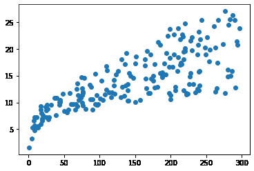
plt.scatter(data.TV,data.sales)

<matplotlib.collections.PathCollection at 0x2a67f0e33d0>

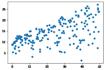
plt.scatter(data.radio,data.sales)

<matplotlib.collections.PathCollection at 0x2a67f1e6520>

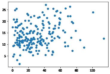
plt.scatter(data.newspaper,data.sales)

<matplotlib.collections.PathCollection at 0x2a67f337ca0>

x = data.iloc[:, 0:-1]  # 取所有行，以及除去最后一列的数据

x

	TV	radio	newspaper
1	230.1	37.8	69.2
2	44.5	39.3	45.1
3	17.2	45.9	69.3
4	151.5	41.3	58.5
5	180.8	10.8	58.4
...	...	...	...
196	38.2	3.7	13.8
197	94.2	4.9	8.1
198	177.0	9.3	6.4
199	283.6	42.0	66.2
200	232.1	8.6	8.7

200 rows × 3 columns

y = data.iloc[:,-1]  # 取所有行以及最后一列的数据
y

1      22.1
2      10.4
3       9.3
4      18.5
5      12.9
       ... 
196     7.6
197     9.7
198    12.8
199    25.5
200    13.4
Name: sales, Length: 200, dtype: float64

model = tf.keras.Sequential(
    # 列表形式[]，几个列表元素就是有多少个感知器
    # 10表示输出的单元的个数，3表示输入的三个维度，activation就是中间层的激活，
    # 1表示第二层输出的单元个数，因为第二层就是最后的输出层，所以就是输出的结果是一个
    [tf.keras.layers.Dense(10,input_shape=(3,),activation='relu'),  
    tf.keras.layers.Dense(1)
    ]
) 

model.summary()

Model: "sequential"
_________________________________________________________________
Layer (type)                 Output Shape              Param #   
=================================================================
dense (Dense)                (None, 10)                40        
_________________________________________________________________
dense_1 (Dense)              (None, 1)                 11        
=================================================================
Total params: 51
Trainable params: 51
Non-trainable params: 0
_________________________________________________________________

• 第一行的param中为40是因为有三个输入再加一个偏置b也就是\(w_i1x_1+w_i2x_2+w_i3x_3+bi=y_i\)
• 第二行有11个参数是因为十个输入再加上一个偏置!

# 训练模型
model.compile(
    optimizer='adam',# adam是常用的优化方法
    loss='mse'
)

model.fit(x,y,epochs=100)

Epoch 91/100
7/7 [==============================] - 0s 833us/step - loss: 3.6655
Epoch 92/100
7/7 [==============================] - 0s 834us/step - loss: 3.6252
Epoch 93/100
7/7 [==============================] - 0s 1000us/step - loss: 3.5899
Epoch 94/100
7/7 [==============================] - 0s 833us/step - loss: 3.5679
Epoch 95/100
7/7 [==============================] - 0s 1ms/step - loss: 3.5273
Epoch 96/100
7/7 [==============================] - 0s 833us/step - loss: 3.5049
Epoch 97/100
7/7 [==============================] - 0s 834us/step - loss: 3.4880
Epoch 98/100
7/7 [==============================] - 0s 1000us/step - loss: 3.4627
Epoch 99/100
7/7 [==============================] - 0s 667us/step - loss: 3.4396
Epoch 100/100
7/7 [==============================] - 0s 1ms/step - loss: 3.4226

<keras.callbacks.History at 0x2a67fc77ee0>

test = data.iloc[:10,0:-1] # 对前十个数据进行预测

model.predict(test)

array([[22.26979  ],
       [14.242942 ],
       [ 8.892993 ],
       [18.704414 ],
       [13.689433 ],
       [ 6.2554317],
       [11.340095 ],
       [10.898435 ],
       [ 1.2222604],
       [11.607856 ]], dtype=float32)

data.iloc[:10,-1]

1     22.1
2     10.4
3      9.3
4     18.5
5     12.9
6      7.2
7     11.8
8     13.2
9      4.8
10    10.6
Name: sales, dtype: float64