Natural Language Processing

NLP before LLM

Context-free Grammar

A context-free grammar (CFG) contains a set of production rules, which are rules saying how each nonterminal can be replaced by a string of terminals and non-terminals. Derivations are a sequence of steps where non-terminals are replaced by the right-hand side of a production rule in the CFG.

Given $G$ as a CFG. The language of $G$, denoted as $\mathcal{L}(G)$, is the set of strings derivable by $G$ (from the start symbolt). A language $L$ is called a context-free language (CFL) if there is a CFG $G$ such that $L=\mathcal{L}(G)$.

Theorem. Every regular language (regular expressions, regex), is context-free, but not vice versa.

Example $L_0$: Natural Language.

Clearly, CFG is (usually) not perfect: $L_0$ could cover more than the language you really want, but it is already useful for parsing.

A CFG is in Chomsky normal form (CNF) if it is $\varepsilon$-free and if in addition Chomsky normal form each production is either of the form $A\to B\;C$ or $A\to a$. ($A\; B\; C$ can be the same symbol)

Theorem. Any context-free grammar can be converted into a CNF.

Given a CFG, syntactic parsing refers to the problem of mapping from a sentence to its parse tree. We can use dynamic programming to parse a sentence (CKY parsing). However, there coult be ambiguity. To resolve ambiguity, we can use probabilistic CFG (PCFG), which associates a probability with each production rule. The probability of a parse tree is the product of the probabilities of all the production rules used in the tree.

Latent Semantic Analysis

The term-document (TD) matrix $W_{td}\in\mathbb{R}^{m\times n}$, where $m$ is the number of terms and $n$ is the number of documents. Each entry $W_{td}(ij)$ is the frequency of term $i$ in document $j$. i.e., rows are terms and columns are documents.

Since the co-occurrence statistics might be sparse, instead of directly using ܹ$W_{td}$, we want to infer a "latent" vector representation (row vec) for the words/documents which satisfies:

\[W_{td}(ij)\approx \max(lv(w_i)lv(d_j)^\top,0). \]

To achieve this, we can use SVD. Besides, in order to make related words have related vectors, we need to use low-rank approximation. That is, we compute the SVD of $W_{td}$ and keep only the top $k$ singular values and corresponding singular vectors.

Another problem is that SVD would pay too much attention to the high-freq words. So we apply TF-IDF normalization. That is, we replace $W_{td}(ij)$ by $tf(i,j)\cdot idf(i)$, where

Term frequency ($tf(i,j)$):

\[\frac{\text{\# of times word }i\text{ appears in doc }j}{\text{\# of words in doc }j}. \]

Inverse document frequency ($idf(i)$), smoothed version:

\[\log \left(\frac{\text{\# of docs} + 1}{\text{\# of docs containing word }i + 1}\right)+1. \]

Hidden Markov Model

Gaussian Mixture Model

Consider a mixture of $k$ Gaussian distributions. Each Gaussian has its own mean $\mu_c$, variance $\sigma_c$, and mixture weight $\pi_c$. The probability density function of the mixture is

\[p(x)=\sum_{c=1}^k \pi_c \mathcal{N}(x;\mu_c,\sigma_c). \]

Equivalent "latent variable" form:

\[\begin{align*} p(z=c)&=\pi_c\\ p(x|z=c)&=\mathcal{N}(x;\mu_c,\sigma_c). \end{align*} \]

Given a dataset $X$ that is i.i.d. drawn from GMM, we want to estimate the parameters $\theta=\{\pi_c,\mu_c,\sigma_c\}_{c=1}^k$.

The Expectation-Maximization Algorithm

The EM algorithm is used to find maximum likelihood parameters of a statistical model. Formally, we want to optimize $\theta$ to maximize the log-likelihood of the observed data:

\[\log p(X|\theta)=\log \sum_Z p(X,Z|\theta). \]

Consider any $q$ distribution, applying Jensen's inequality gives

\[\begin{align*} \log \sum_Z p(X,Z|\theta)=&\ \log \sum_Z q(Z)\frac{p(X,Z|\theta)}{q(Z)}\\ \ge&\ \sum_Z q(Z)\log p(X,Z|\theta)+\text{H}(q), \end{align*} \]

where $\text{H}(q)=-\sum_Z q(Z)\log q(Z)$ is the entropy of $q$.

Denote the current parameter as $\theta'$. Set $q(Z)=p(Z|X,\theta')$ and let the above objective be $Q(\theta|\theta')$. One can verify that

\[\log p(X|\theta)= Q(\theta|\theta')+\text{KL}(q(Z)||p(Z|X,\theta)). \]

When $\theta'$ is close to $\theta$, the KL divergence is small, and maximizing $Q(\theta|\theta')$ is approximately maximizing $\log p(X|\theta)$.

The EM algorithm iteratively performs the following two steps until convergence. In the $k$-th iteration:

E-step: Let $\theta_k$ be the current parameter estimate. Compute $$q(Z)=p(Z|X,\theta_k)=\frac{p(Z,X|\theta_k)}{p(X|\theta_k)}.$$

For GMM, we have $\theta=\{\pi_c,\mu_c,\sigma_c\}_{c=1}^k$, so when $Z=c,X=x_i$, it's

\[r_{ic}=\frac{\pi_{c}\mathcal{N}(x_i;\mu_{c},\sigma_{c})}{\sum_{c'} \pi_{c'} \mathcal{N}(x_i;\mu_{c'},\sigma_{c'})}. \]

M-step: We fix $q(Z)$ and optimize $\theta$ to maximize $Q(\theta|\theta_k)$. That is, minimize

\[\sum_i\sum_c r_{ic}\log \left(\pi_c\mathcal{N}(x_i;\mu_c,\sigma_c)\right). \]

Let $m_c=\sum_i r_{ic}$ and $m=\sum_c m_c$. Solving the optimization problem gives

\[\begin{align*} \pi_c=&\ \frac{m_c}{m},\\ \mu_c=&\ \frac{1}{m_c}\sum_i r_{ic} x_i,\\ \sigma_c=&\ \frac{1}{m_c}\sum_i r_{ic}(x_i-\mu_c)^2. \end{align*} \]

Hidden Markov Model

Given a sentence, we want to identify the grammatical category of each word. We can use HMM to model the problem. Let $O$ be the observed words, and $Q$ be the hidden states (grammatical categories). The model parameters include:

Initial state distribution: $\pi_i=p(q_1=i)$;
State transition distribution: $a_{ij}=p(q_{t+1}=j|q_t=i)$;
Emission distribution: $b_i(o_t)=p(o_t|q_t=i)$.

If we're given the parameters $A,B,\pi$, we can calculate the probability of an observation sequence $O$ using the forward algorithm, and we can find the most likely hidden state sequence $Q$ using the Viterbi algorithm. They both use dynamic programming.

Thus, for supervised learning, we just need to count & normalize; for unsupervised learning, we can use the EM algorithm with $Q$ as hidden states.

Generally, we have Directed Graphical Models (DGM):

Let $G$ be a DAG with vertices $V=\{x_1,...,x_d\}$. If $P$ is a distribution for $V$ with probability function $p(x)$, we say that $P$ is Markov to $G$, or that $G$ represents $P$, if

\[p(x) = \prod_{j=1}^{d} p(x_j \mid \pi_{x_j}) \]

where $\pi_{x_j}$ is the set of parent nodes of $X_j$.

N-gram

A Language Model assigns a probability of any sequence of words. That is,

\[\sum_{W\in V^*} p(W)=1. \]

A good LM should put high probability to more "likely" sentences.

Uni-gram LM: $P(w_1w_2\cdots w_T)=P(w_1)P(w_2)\cdots P(w_T).$
Bi-gram LM: $P(w_1w_2\cdots w_T)=P(w_1)P(w_2|w_1)P(w_3|w_2)\cdots P(w_T|w_{T-1}).$
Tri-gram LM: $P(w_1w_2\cdots w_T)=P(w_1)P(w_2|w_1)P(w_3|w_1w_2)\cdots P(w_T|w_{T-2}w_{T-1}).$
N-gram LM: $P(w_1w_2\cdots w_T)=\prod_{t=n}^T P(w_t|w_{t-(n-1)}\cdots w_{t-1}).$

There are two special tokens that are very useful in building a LM.

The end-of-sentence token: <eos>, tells where a sentence could end.
The out-of-vocabulary token: <unk>, replaces rare words (e.g., appearing only once in the training corpus).

In order to build a LM, we need to estimate the conditional probabilities $P(w_t|w_{t-(n-1)}\cdots w_{t-1})$. The straightforward way is to directly count & normalize. However, this would lead to the zero-frequency problem (cannot create new sentences). Ways to solve it:

Add-k smoothing: $$P(w_t|w_{t-(n-1)}\cdots w_{t-1})=\frac{\text{count}(w_{t-(n-1)}\cdots w_{t-1}w_t)+k}{\text{count}(w_{t-(n-1)}\cdots w_{t-1})+k|V|}.$$
Linear interpolation: $$P(w_t|w_{t-(n-1)}\cdots w_{t-1})=\lambda_n P(w_t|w_{t-(n-1)}\cdots w_{t-1})+\lambda_{n-1} P(w_t|w_{t-(n-2)}\cdots w_{t-1})+\cdots+\lambda_1 P(w_t),$$
where $\sum_{i=1}^n \lambda_i=1$.
Backoff: $$P(w_t|w_{t-(n-1)}\cdots w_{t-1})=\begin{cases} \frac{\text{count}(w_{t-(n-1)}\cdots w_{t-1}w_t)}{\text{count}(w_{t-(n-1)}\cdots w_{t-1})}, & \text{if } \text{count}(w_{t-(n-1)}\cdots w_{t})>0 \ \alpha(w_{t-(n-2)}\cdots w_{t-1})P(w_t|w_{t-(n-2)}\cdots w_{t-1}), & \text{otherwise} \end{cases},$$
where $\alpha(w_{t-(n-2)}\cdots w_{t-1})$ is a normalization factor.

Given a test set $W$, we define the LM's perplexity to be

\[PPL(W)=2^{-l}, \text{ where }l=\frac{\log_2 (P(W)) }{\text{token\_len}(W)}. \]

Perplexity cares more about diversity than quality.

Word2vec

In the LSA section, we obtained word vectors by decomposing the term-document matrix; In this section, we will talk about another approach based on prediction.

Skip-gram: learn representations that predict the context given a word.
\[p_{\text{skip-gram}}(x_{t-s}...x_{t+s}|x_t)=\prod_{-s\le j\le s,j\ne0} p(x_{t+j}|x_t) \]
where
\[p(\text{out}|\text{in})=\frac{\exp(u_\text{out}\cdot w_\text{in})}{\sum_{v\in V} \exp(u_v\cdot w_\text{in})}. \]
CBOW (Continous Bag-of-Words): learn representations that predict a word given context.

\[p_{\text{CBOW}}(x_t|x_{t-s}...x_{t+s})=p\left(x_t\bigg |\sum_{-s\le j\le s,j\ne0} x_{t+j}\right) \]

The objective function of skip-gram is

\[\sum_{t=1}^T \sum_{-s\le j\le s,j\ne0} \log p(x_{t+j}|x_t). \]

Take gradient for the input embedding matrix of skip-gram, and apply SGD, we get:

\[w_x\gets w_x+\eta\left(u_y-\sum_{z\in V} p(z|x)u_z\right). \]

However, computing $\sum_{z\in V} p(z|x)u_z$ is expensive. Negative sampling is a way to approximate it. The idea is to sample a few negative examples from a noise distribution $P_n$, and only update the weights for the positive example and the negative examples. The new objective function is

\[\log \sigma(u_y\cdot w_x)+\sum_{i=1}^k \mathbb{E}_{y_i\sim P_n}[\log \sigma(-u_{y_i}\cdot w_x)]. \]

Neural Network Language Model

Basics

Framework

General recipe for classification: Encode, Predict, Train.

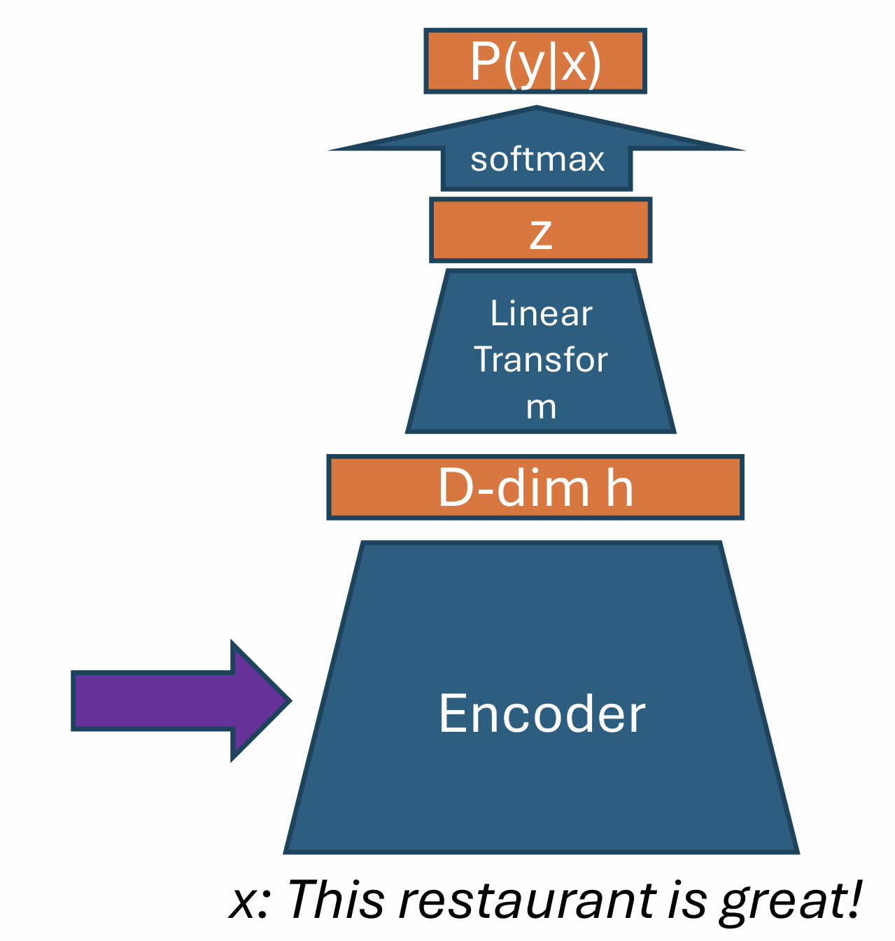
How to encode?

Bag of words:

a $|V|$-dim vector, the $i$-th dimension indicates whether the i-th word in $V$(vocabulary) exists in x.

Since $|V|$ could be very large, we can multiply it with a $D$-by-$|V|$ word embedding matrix $W$. The difference with LSA and word2vec is that here the word embedding matrix is treated as part (the first layer) of the parameters of the NN model.

Next, we want to predict the label. Neural networks are good at this.

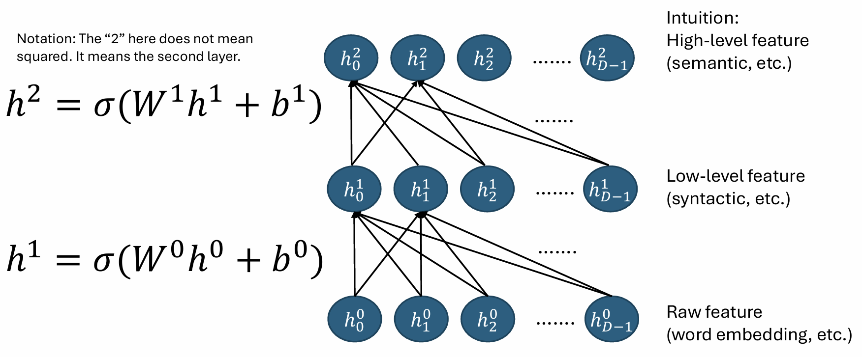
A neural unit (aka. neuron) is a function that can extract low-level features from the input:

\[y=\sigma(w^Tx+b). \]

A layer of $D$ neurons consists a hidden layer. Multiple hidden layers can be stacked to form a multi-layer perceptron (MLP), which is the simplest type of deep neural network.

Choice of activation function:

Sigmoid: $y=\frac{1}{1+\exp(-x)}$.
ReLU: $y=\max(0,x)$.

Back-propagation

Suppose $\mathbf{f}:\mathbf{R}^{n}\rightarrow\mathbf{R}^{m}$ is a function such that each of its first-order partial derivatives exist on $\mathbf{R}^{n}$. This function takes a point $\mathbf{x}\in\mathbf{R}^{n}$ as input and produces the vector $\mathbf{f}(\mathbf{x})\in\mathbf{R}^{m}$ as output. Then the Jacobian matrix of $\mathbf{f}$ is defined to be an $m\times n$ matrix, denoted by $\mathbf{J}$, whose $(i,j)$th entry is $\mathbf{J}_{ij}=\frac{\partial f_{i}}{\partial x_{j}}$, or explicitly

\[\frac{\partial \mathbf{f}}{\partial \mathbf{x}}=\left[\begin{array}{ccc} \frac{\partial\mathbf{f}}{\partial x_{1}} & \cdots & \frac{\partial\mathbf{f}}{\partial x_{n}} \end{array}\right]=\left[\begin{array}{c} \nabla^{\mathrm{T}} f_{1} \\ \vdots \\ \nabla^{\mathrm{T}} f_{m} \end{array}\right]=\left[\begin{array}{ccc} \frac{\partial f_{1}}{\partial x_{1}} & \cdots & \frac{\partial f_{1}}{\partial x_{n}} \\ \vdots & \ddots & \vdots \\ \frac{\partial f_{m}}{\partial x_{1}} & \cdots & \frac{\partial f_{m}}{\partial x_{n}} \end{array}\right] \]

where $\nabla^{\mathrm{T}}f_{i}$ is the transpose (row vector) of the gradient of the $i$ component.

For example,

$\frac{\partial W h+b}{\partial h}=W$
$\frac{\partial \log P(y|x)}{\partial z}=\frac{\partial \log \text{softmax}(z)[y]}{\partial z}=(\tilde{y}-\text{softmax}(z))$ , where $\tilde{y}$ is the one-hot encoding of ground-truth label y.
$\frac{\partial\sigma(a)}{\partial a}=\text{diag}[\sigma(a)\odot(1-\sigma(a))],$ where $\odot$ is element-wise multiplication.

Finally, the chain rule: if $\mathbf{f}:\mathbf{R}^{n}\rightarrow\mathbf{R}^{m}$ and $\mathbf{g}:\mathbf{R}^{m}\rightarrow\mathbf{R}^{p}$, then

\[\frac{\partial \mathbf{g}}{\partial \mathbf{x}}=\frac{\partial \mathbf{f}}{\partial \mathbf{x}}^\top\frac{\partial \mathbf{g}}{\partial \mathbf{f}}. \]

The dropout regularization

Dropout is a regularization technique for neural networks that randomly drops a unit (along with connections) at training time with a specified probability $p$ (0.3 or 0.5).

This masking is randomly sampled for each mini-batch. At test time, all units are present, but with weights scaled by $p$.

Intuition: Instead of train one model, we are training an ensemble of models. And average them during evaluation (for better generalization).

RNN, GRU and Bi-directional RNN

From FNN to RNN

(F)NN version of trigram model:

\[L=\sum_{(w_{i-2},w_{i-1},w_i)\in \text{data}} \log P(w_i|w_{i-2},w_{i-1}), \]

where

\[P(w_i|w_{i-2},w_{i-1})=\text{NN}(w_{i-2},w_{i-1})[w_i]. \]

To speed-up the output layer computation $D|V|$, we cluster the words into $\sqrt{V}$ clusters. We decompose the prediction of a token into first its class, and then the token inside that class.

However, the FNNLM only encodes a very limited context.

RNN defines an efficient flow of computation to encode the whole history.

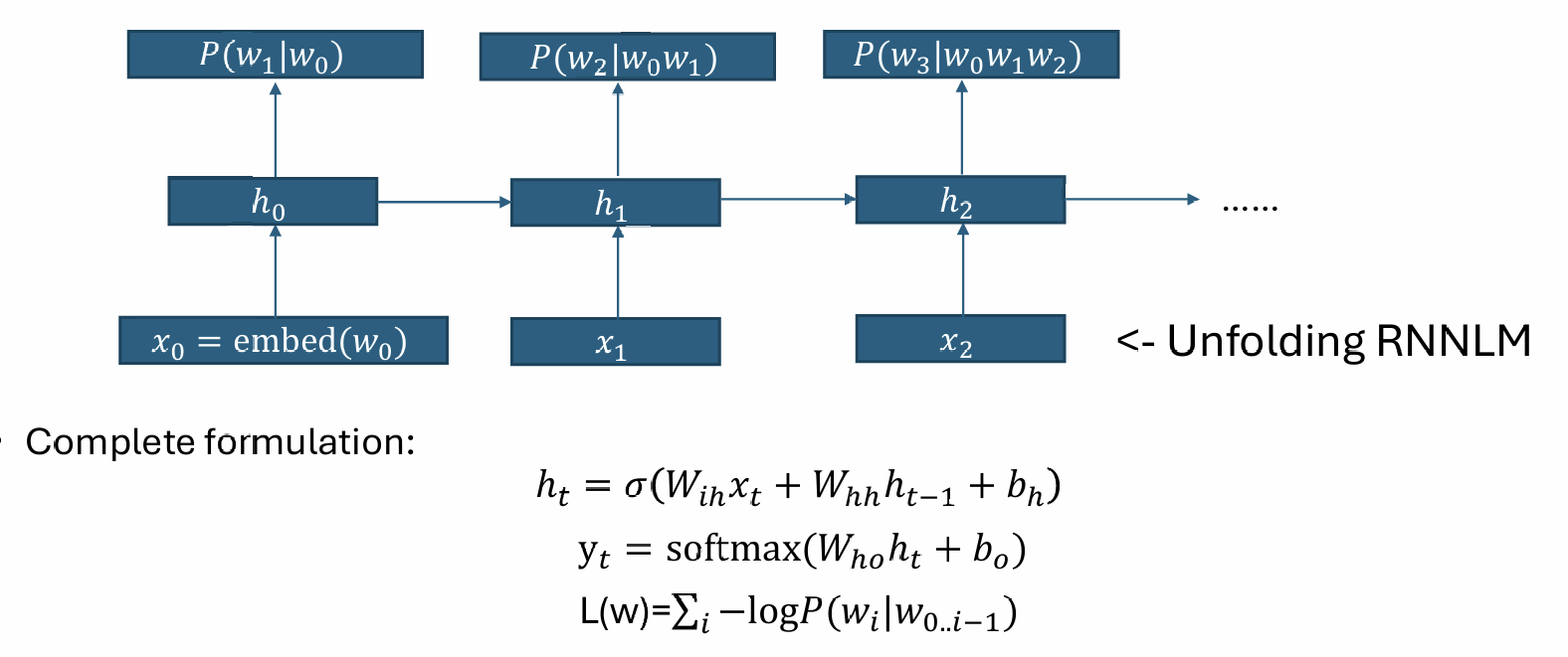
Sampling with RNNLM: sample the next token, and feed it to the next timestep;
RNN for text classification: the last hidden state can beregarded as an encoding of the whole, and fed to a classifier.

In Back-propagation through time (BPTT), we could meet two seriousproblems: gradient exploding and gradient vanishing.

To solve the exploding problem, we can apply gradient clipping:

\[\text{clip}(\nabla L)=\min\left\{1,\frac{\gamma}{\|\nabla L\|_2}\right\}\nabla L. \]

LSTM & GRU

The LSTM (long-short term memory) network was used to solve the vanishing gradient problem. LSTM is quite complicated! We will discuss GRU because it’s simpler and has the same core idea.

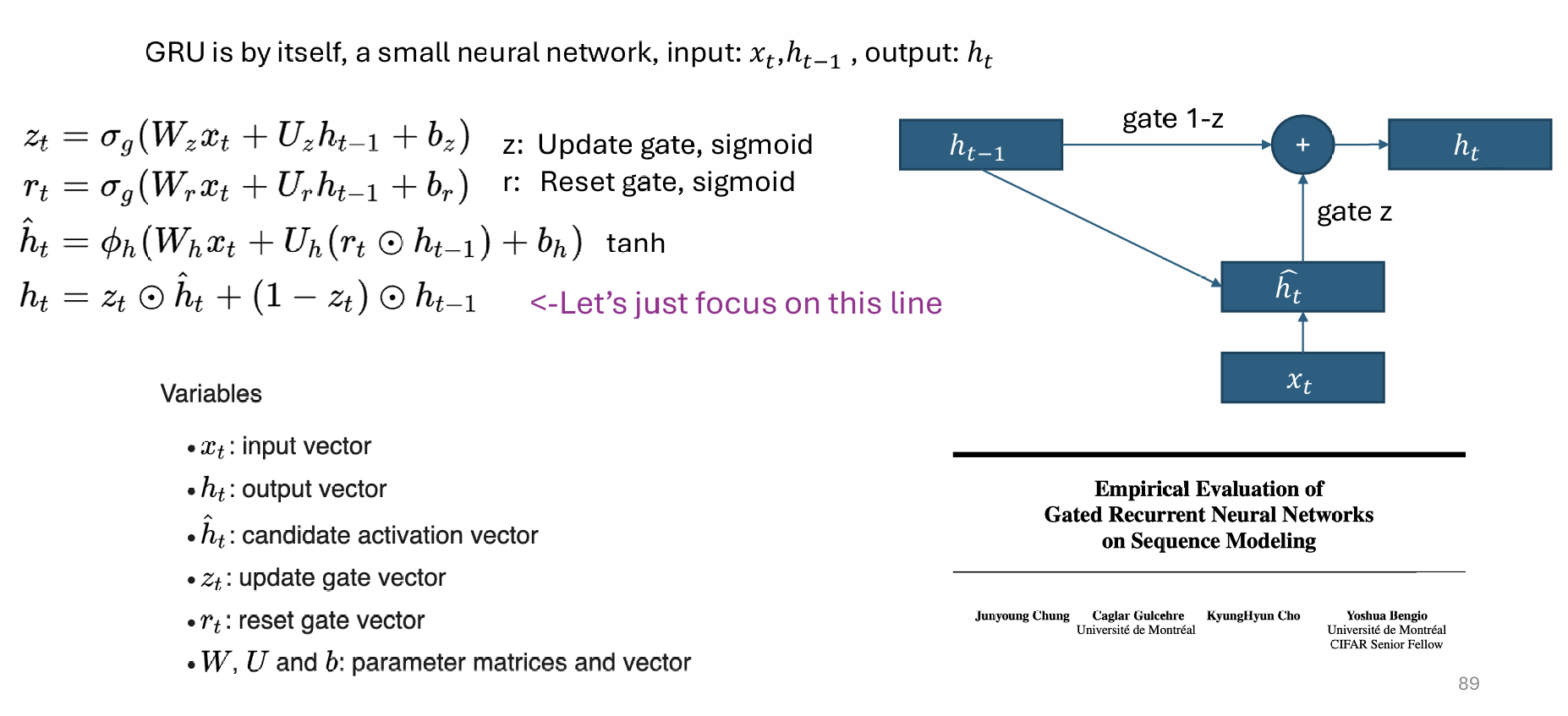
There is a path doesn't involve any weight matrix, alleviates gradient vanishing.

Bi-directional RNN

In uni-directional RNN, $h_t$ has context from the "left". For some applications, it would be useful if $h_t$ has bi-directional context.

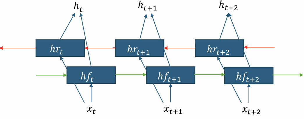
For Seq2seq tasks (e.g., machine translation), we can use a bi-rnn encoder for the input sequence, and use a uni-rnn decoder for the output. For decoding, we can use beam search to find the top-k most likely output sequences.

Attention

Currently, all information in the input is condensed into a single vector. However, in tasks like MT, we may want to pay attention to different parts of the input in different timesteps.

The attention module isproposed to learn this alignment in an end-to-end fashion.

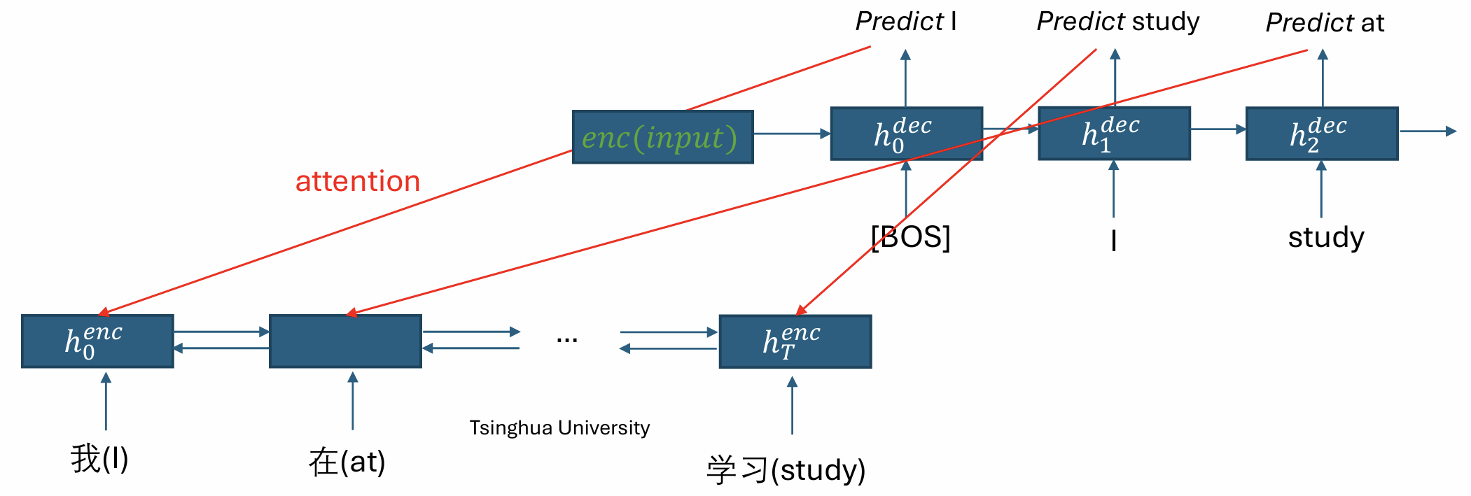
The attention works as follows: For each decoding step $t$,

Compute attention scores: $\hat{a}_{t,i}= (h_i^{\text{enc}})^\top W_a h_{t-1}^{\text{dec}}$.
Get attention weights: $a=\text{softmax}(\hat{a}_t)$.
Reweight encoder hidden states: $c_t=\sum_i a_{t,i} h_i^{\text{enc}}$.

For several years, attention is used in combination with RNN. Very successful. Until 2017, transformer comes, and RNN becomes obsolete.

Text Classification

Approach

RNN (or LSTM)

Perform better for hard tasks (could be the default choice).

FastText for + Feedforward nets for classification

Average the (pretrained) embeddings of $n$-gram features to form the hidden variable. Linear layer followed by softmax for classification.
Very fast (small model). Can run on CPUs. Reasonable performance. Popular for many industry applications.

CNN with variable length

For each convolution kernel, apply max-pooling over the whole sequence to get a fixed-length vector.
Easier to train (no gradient problem).

Recursive neural net

Get the hidden vector of the parent node from the vectors of the children nodes. You can also change the LSTM formulation for a tree.
Useful when high-quality parse trees are available.

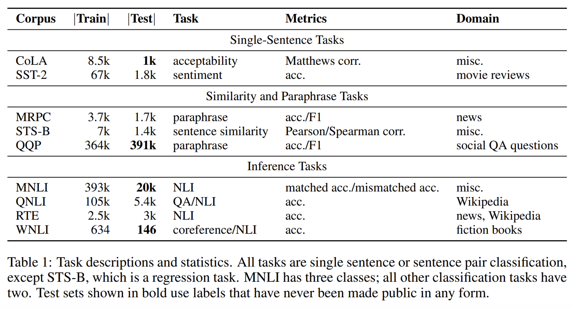
The GLUE Benchmark

Many natural language understanding (NLU) tasks can be posed as a text classification task. And these tasks can be approached by one general (neural) model, but finetuned on the data of each task. So, it would be nice to have a popular benchmark where models can be compared on a set of NLU tasks. And that brings the GLUE benchmark.

The set of tasks is as follows. The majority is not difficult for human.

Interestingly, with BERT and other LLM coming out in 2019, LLMs
got super-human performance on the GLUE tasks. That calls for a harder set of tasks, which brings SuperGLUE. Currently, LLMs get super-human also in SuperGLUE.

ELMo

We have talked about “shallow” word embedding models... ELMo (Embeddings from Language Models) aims to build deep contextualized word representation.

The model is a multi-layer bi-directional LSTM. Its objective is to predict the next word in both directions independently. Showed strong performance on the GLUE tasks.

Subword Tokenization

Up to now we have assumed that we tokenize each sentence by words. In that case, the representation for rare words (or <unk>) would be bad. A better approach is to use subword units. Language (on the internet) is evolving, a fixed morphology might not be optimal. We nees a data-centric ways to automatically construct subword tokenization.

The byte pair encoding (BPE) tokenization algorithm is as follows: (used in the GPT and LLaMA model series)

Start with a unigram vocabulary of all characters in the data.
Each iteration: In the data, find the most frequent pair, merge it, and add to the vocabulary.
Stop when vocabulary is of pre-determined size (e.g., 50k).

Generation

VAE-LM

In RNNLM, we generate token-by-token. However, that’s not the way we human generate a sentence.

In VAE, we want to first generate a continuous vector $z$ representing the latent semantic of the whole sentence, and then we generate $x$ from $z$ (denoted as model $p$). At the same time, we want a posterior model $q_\theta(z|x)$ which we can use as a encoder.

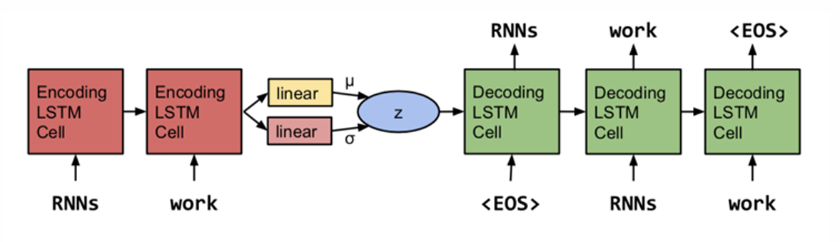
Generation:

Sample $z$ from prior $p(z)$;
Sample $x$ from our generative model $P_\theta(x|z)$.

Training: The "ELBO" objective (maximize)

\[L(\theta; x)=-\text{KL}(q_\theta(z|x)||p_\theta(z))+\mathbb{E}_{q_\theta(z|x)}[\log p_\theta(x|z)]\le \log p_\theta(x). \]

here both the prior $p$ and the posterior $q$ are Gaussian. The term $-\text{KL}(q_\theta(z|x)||p(z))$ is a regularization term, preventing $q$ from deviating too much from the prior $p(z)$; the term $\mathbb{E}_{q_\theta(z|x)}[\log p_\theta(x|z)]$ is the reconstruction loss, encouraging $p_\theta(x|z)$ to reconstruct $x$ well from $z$ sampled from $q_\theta(z|x)$.

We have the following with relationship with the marginal log-prob:

\[\log p_\theta(x)=L(\theta;x)+\text{KL}(q_\theta(z|x)||p_\theta(z|x)). \]

So, when we are maximizing ELBO, we are also learning a good posterior $q$.

Problem:

Think about training, the reconstruction loss involves a sampling operation from the parameterized $q$, which we can not directly back-prop.
Solution: We can use the reparameterization trick: sample $\epsilon$ from a fixed distribution, and let $z=\mu+\sigma\odot \epsilon$. Then we can back-prop through $\mu$ and $\sigma$.
In VAE-LM training, KL term quickly decrease to zero (throwing away latent information). Potential reason: decoder is strong and the KL term is too easy to optimize.
Solution:
- KL cost annealing: We add a variable weight to the KL term in the cost function at training time. At the start of training, we set that weight to zero, then gradually increase.
- Input word dropping: A natural way to weaken the decoder is to remove some or all of this conditioning information during learning, forcing the model to rely on the latent vector.
- Bag-of-words loss: In parallel, train the decoder network to predict the bag-of-words in the response $x$.

As pure autoregressive LLMs are tuned to have stronger instruction-following ability, consistency, and showing strong representation power, VAE LM seem to be less attractive recently. Also in computer vision, VAE are being replaced by GAN or diffusion.

MLE

Given a dataset of text sequences, we want to learn a language model $P_\theta$ by maximizing the log-likelihood:

\[L(\theta)=\log P_\theta(W)=\sum \log P_\theta(w_t|w_{<t}). \]

Teacher Forcing:

Training: $\log P(W^D)=\sum \log P(w_t^D|w_{<t}^D)$
Generation: $w_t^M\sim P_\theta(w_t|w_{<t}^M)$, $M$ refers to model generation.

The open-ended generation performance of MLE-trained LM are very poor. Researchers think teacher forcing in MLE training is to blame!

The exposure bias hypothesis: Due to the exposure to ground-truthprefix, the model is biased to only perform well during training, but not generation.

So we need to train the model in another way.

GAN

In GAN,there is noteacher forcing (the training is directly applied to model samples):

\[\min_G \max_D \mathbb{E}_{W\sim p_{\text{data}}}[\log D(W)]+\mathbb{E}_{W\sim P_\theta}[\log(1-D(W))]. \]

However, if $G$ is a standard RNNLM, we can't directly apply GAN for language generation, since the sampling operation is not differentiable. To solve this, we may use two techniques:

The Gumbel-softmax reparameterization:

Discrete sampling:

\[z=\text{one\_hot}(\arg\max_i[g_i+\log\pi_i]), \]
where $g_i$ are i.i.d. samples from $\text{Gumbel}(0,1)$ distribution.

Continuous relaxation:

\[y_i=\frac{\exp((g_i+\log \pi_i)/\tau)}{\sum_j \exp((g_j+\log \pi_j)/\tau)}. \]
In addition, we may want our encoding to really be one-hot during training, so we can use the straight-through estimator: in the forward pass, we use $z$ for the next step computation, but in the backward pass, we use the gradient of $y$ to approximate that of $z$.
The reinforce trick (from policy gradient)

\[\begin{aligned} &\arg\max_\theta \ \mathbb{E}_{y \sim P_\theta(y|x)} [r(x, y)] \\[6pt] \nabla_\theta \ \mathbb{E}_{y \sim P_\theta(y|x)} [r(x, y)] &= \nabla_\theta \sum_y r(x, y) P_\theta(y|x) \\[6pt] &= \sum_y r(x, y) \nabla_\theta P_\theta(y|x) \\[6pt] &= \sum_y r(x, y) P_\theta(y|x) \nabla_\theta \log P_\theta(y|x) \\[6pt] &= \mathbb{E}_{y \sim P_\theta(y|x)} [r(x, y) \nabla_\theta \log P_\theta(y|x)] \end{aligned} \]

However, GAN training for text generation is very unstable and hard to tune. Actually, MLE with tuned temperature is better. (Trade-off between quality and diversity.)

Why MLE training emphasizes diversity? KL divergence in MLE learns the diversity. Also researchers find that exposure bias is not that serious. MLE with sampling algorithm is already good enough.

Sampling methods

Three popular sampling algorithms:

Top-K: $\hat{p_i}=\frac{1}{Z}p_i\cdot\mathbf{1}(i\in \text{Top-K})$.
Nucleus (top-P): $\hat{p_i}=\frac{1}{Z}p_i\cdot\mathbf{1}(\sum_{j<i} p_j<P)$, where $i$ are sorted by $p_i$ in descending order.
Temperature (T): $\hat{p_i}=\frac{1}{Z}\exp(\log p_i/T)$.

Common property:

The order of elements are preserved

\[\hat{p_i}>\hat{p_j}\Leftrightarrow p_i>p_j. \]
The entropy of the distribution are reduced

\[H(\hat{p})<H(p). \]
The slope of the non-zero elements are preserved

\[\frac{\log p_i-\log p_j}{\log p_j-\log p_k}=\frac{\log \hat{p_i}-\log \hat{p_j}}{\log \hat{p_j}-\log \hat{p_k}} \]
for any $\hat{p_i},\hat{p_j},\hat{p_k}>0$.

We hypothesize that:

Sampling algorithms that satisfy all three properties should be at least as good as the top-k/nucleus/tempered sampling in the Q-D trade-off.
Sampling algorithms that violate at least one of the properties won’t be as good.

We can not prove it, but we can design some new sampling algorithm to test this hypothesis.

The degenerated behaviors

Let's look again at the MLE objective

\[\arg\min_\theta \text{KL}(p_{\text{data}}||P_\theta)=\arg\min_\theta \mathbb{E}_{W\sim p_{\text{data}}}[-\log P_\theta(W)]. \]

We have taught the model what to say, but we did not teach what not to say!

Bad behavior:

The repetition problem for beam-search
The generic response problem for chat-bots

Reason: Combined with MLE training, when the model is not sure about what to say, it degrades to some simple and "safe" pattern in data.

Tackling bad behaviors:

Biased decoding (for repetition)

\[\hat{p_i}=\frac{1}{Z}\exp(p_i/(T\cdot I(i\in g))), \]
where $g$ refers to the set of generated tokens and $I(c)=\theta>1$ if condition $c$ is true else $1$.
Unlikelihood training (for repetition)

\[L^t(\theta,C^t)=-\alpha\cdot\sum_{c\in C^t} \log(1-P_\theta(c|x_{<t}))-\log P_\theta(x_t|x_{<t}), \]
where $C^t=\{x_1,...x_{t-1}\}- \{x_t\}$.
The MMI criterion (for generic response)

\[\hat{T}=\arg\max_T \{\log P_\theta(T|S)-\log P_\theta(T)\}. \]
where $S$ is the history.
Negative training (for generic response)

We can dynamically count the frequency of decoded response from the model during training, and assign negated gradients to those most frequent samples (denoted as $y_{\text{neg}}$:

\[L(\theta)=-\log P_\theta(y_{\text{pos}}|x_{\text{pos}})+\log P_\theta(y_{\text{neg}}|x_{\text{neg}}). \]

The degenerated behaviors (like repetitions) are becoming better as model capacity increases. However, hallucinations emerges as a serious problem.

Transformer

Self-attention

With three weight matrices $W_q,W_k,W_v$, we compute the query $q$, key $k$, and value $v$ for each $x$ via linear transformation:

\[q_i=W_qx_i,\quad k_i=W_kx_i,\quad v_i=W_vx_i. \]

Then we compute the attention scores by dot-product of query and key vectors. Scale by
$\frac{1}{\sqrt{\dim k}}$ and apply softmax:

\[a_{i*}=\text{softmax}\left(\frac{q_i^\top k_*}{\sqrt{\dim k}}\right). \]

And then we get the outputs by weighting the value vectors:

\[z_i=\sum_j a_{ij} v_j. \]

Multi-head attention: use multiple sets of $W_q,W_k,W_v$ to get multiple outputs, and concatenate them together.

Transformer Block

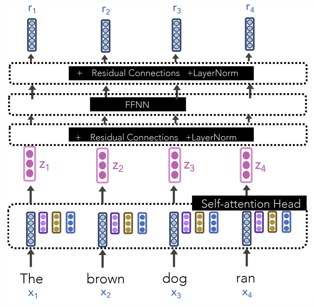
$f_{\text{residual}}(x, F)=F(x)+x, \text{LayerNorm}(h)=\alpha\frac{h-\text{mean}(h)}{\text{std}(h)}+\beta$.

Combine them:

\[h_{\text{out}}=F(\text{LayerNorm}(x))+x \]

where $F$ is either the multi-head attention or the FFNN.

Last problem: Without RNN, attention alone does not have order information! We need positional encoding, i.e., we add the following vector to each input embedding:

\[p_i=[\sin(i/10000^{2/d}),\cos(i/10000^{2/d}),\sin(i/10000^{4/d}),\cos(i/10000^{4/d}),...]. \]

Rotary position embedding: we want

\[\langle f_q(x_m,m),f_k(x_n,n)\rangle=g(x_m,x_n,m-n), \]

so we have (for $2$-d)

\[f_{q,k}(x_m,m)=\begin{bmatrix}\cos m\theta & -\sin m\theta \\ \sin m\theta & \cos m\theta \end{bmatrix}\begin{bmatrix}W_{q,k}^{(11)} & W_{q,k}^{(12)} \\ W_{q,k}^{(21)} & W_{q,k}^{(22)} \end{bmatrix}\begin{bmatrix}x_m^{(1)} \\ x_m^{(2)} \end{bmatrix}. \]

Generalize to higher dimensions by applying the rotation to each pair of dimensions.

For transformer models, it is very useful to set a small warmup stage, where we first gradually increase lr from zero to the starting value.

BERT (Transformer encoder)

BERT is a transformer encoder pretrained on large data, and then finetuned on downstream NLU tasks.

MLM and NSP

BERT (Bidirectional Encoder Representations from Transformers) is pretrained on data of 3 billion tokens with self supervised training.

Two major objective used in BERT pretraining:

Masked language modeling (MLM)
Next sentence prediction (NSP)

MLM: Randomly mask 15% of the tokens in each sequence, and ask the model to predict the masked token on the top layer via standard cross-entropy loss.

Problem: If we only add loss for masked tokens, then the transformer would not build
good representations for non-masked tokens.

Heuristic:

For 10% of the time, we replace [M] with a random token.
For another 10% of the time, we do not change the original token.
O.w., the mask token is used.

NSP: In addition to MLM, we also add a [CLS] token and ask BERT to predict whether sentence2 is the next sentence of sentence1. For 50% of the time, a random sentence is used as a negative example.

However, later work empirically shows that NSP is actually not useful in pretraining, and is therefore not used after BERT.

Ignited by the success of BERT… Quickly, a bunch of BERT-like models are proposed and trained…

ALBERT (2019, A Lite BERT …)
RoBERTa (2019, A Robustly Optimized BERT …)
DistilBERT (2019, smaller, faster, lighter version of BERT)
ELECTRA (2020, Pre-training Text Encoders as Discriminators not
Generators)
LongFormer (2020, Long-Document Transformer)

ELECTRA

ELECTRA (Efficiently Learning an Encoder that Classifies Token Replacements Accurately)

Instead of masking the input, our approach corrupts it by replacing some tokens with plausible alternatives sampled from a small generator network. Then, instead of training a model that predicts the original identities of the corrupted tokens, we train a discriminative model that predicts whether each token in the corrupted input was replaced by a generator sample or not.

This new pre-training task is more efficient than MLM because the task is defined over all input tokens rather than just the small subset that was masked out.

Longformer

It is hard to apply transformer on very long sequences because the attention computation scales quadratically with sequence length.

Sliding window attention: Limit the attention a fixed local span of size $w$.

We can add gaps in the window to make it even wider with the same amount of compute. For example, we can use a combination of 2 heads of dilated and other heads with local sliding window.

Longformer is efficient for tasks requiring long documents.

Transformer decoder

BERT-like models are great for sentence/document encoding or deep contextualized word embedding. But you can not directly use it for text generation, or infer the log probability of a given text.

Transformer decoder is designed for text generation. The only difference with transformer encoder is that in the self-attention module, each token can only attend to the previous tokens (including itself). This is implemented by applying a mask before softmax.

Transformer encoder-decoder

For seq2seq tasks (e.g., translation), naturally we can combine transformer encoder and transformer decoder, to construct a transformer encoder-decoder model.

Similar to MLM in BERT (encoder), we can design self-supervised pretraining objective as seq2seq tasks for encoder-decoder models.

Around 2019 and 2020, encoder-decoder LLM (e.g., BART and T5) got very strong performance on seq2seq tasks. However, recently industry LLMs have shifted to decoder-only LLMs (GPT3, GPT4, LLaMA).

Consider a turn-by-turn chat-bot setting, decoder-only naturally handles variable-length text generation and do natural concatenation of history and response. Encoder-decoder needs to build text of variable length and we need to re-encode the whole input again for each turn.

GPT and RLHF

GPT1

We pretrain a transformer decoder AR-LM on large data, and the finetune it on downstream NLU tasks.

Then we take the final-layer embedding of the last token in the text, and add a linear classification head.

GPT2

Train a transformer decoder on a new large-scale dataset of millions of webpages called WebText (8m documents, or 40GB of text).

We want to apply the learned model zero-shot to some downstream language generation task (translation, summarization, QA, etc.).

What does AR-LM do during generation? It predicts the next token, in other words, it continues the language.

So, we can construct some simple prompts like the following:

Translate the following text to French. Text: [ENG TEXT] French:

Even without finetuning, a good-enough LM trained on very general data should give a good continuation of the prompt.

Actually, we are implicitly doing multi-task training during the pretraining.

The generation quality of GPT2 is very good, which is attributed to the top-k sampling algorithm, i.e., only keep the top-k tokens with highest probabilities.

GPT3

175 billion model parameters, trained with next-token prediction.

We have Common Crawl which is from web crawling. It’s super large and the training did not fully cover it. High quality data (such as Wiki) is intentionally repeated multiple times.

In-context learning

Few-shot learning: We have a LM trained on general data, we want to use it for a new seq2seq task. For this task, we only have a few (e.g., 2) natural-language demonstrations.

Before GPT3, the common approach is to finetune the LM on the few examples, i.e., meta-learning. MAML: In the inner loop of each sub-task, we update to a pseudo $\theta'$; In the outer loop, we compute real gradient on the dev-set loss with $\theta'$.

However, with GPT3, we can directly use in-context learning (ICL) to perform few-shot learning without any finetuning! We only need to construct some prompt (also called context or prefix) and ask the LM to do continuation.

Please negate the meaning of the sentence. [<- task description, optional]
I hate NLP => I love NLP; Today’s weather is good => Today’s weather is bad; [<- the demonstrations]
I had a good day => [<- the example for testing (output)]

GPT3 has great ICL ability! We find that GPT3 with ICL has outperformed a strong finetuned BERT model.

Majority and recency bias: In few-shot demonstrations, the model tends to follow the majority pattern, and also tends to follow the most recent demonstration. We can calibrate few-shot prediction by adding "null" demonstration and subtracting the output logit.

Instruction tuning: After pretraining, we finetune the language model on a good amount of "instruction following" data. E.g., FLAN.

Starting at GPT3, the strongest LLM can only be accessed through API calls for prompted generation. Therefore, many research focus on how to build good "prompts" for LLMs, e.g., CoT.

Chain-of-Thought Prompting

In the few-shot demonstrations, add reasoning steps before giving the answer. These reasoning steps are manually written by humans. The model will follow this pattern in the output.

CoT is an emergent ability of model scale. That is, its impact is more pronounced when the model is large (~100B).

We can also prompt LLM to do zero-shot chain-of thought reasoning in a zero shot manner! All we need to do is to add one sentence before the answer:

Let's think step by step.

CoT with self-consistency: Sample multiple reasoning path from the LLM with temperature sampling, and then take a majority voting over the answers!

Tree of thoughts (ToT): Maintain and expand a thought-tree. For each existing step, we prompt the LLM to propose multiple next steps, and also to judge which path (by giving a value) is more promising. The nodes that are judged to be unlikely will be discarded.

Continuous CoT: NL reasoning could be redundant, and continuous thought could take less token steps.

Alignment with Reinforcement Learning Human Feedback

We want to align the LLM to better follow human instructions and be more helpful, honest and harmless.

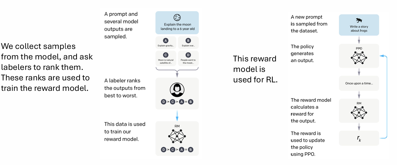
This RLHF pipeline is used to train GPT3.5.

Reward modeling + RL

We use the Bradley-Terry model to describe the distribution of human preferences $p^*$. We train a reward model $r$, the probability of preferring $y_1$ over $y_2$ is

\[P(y_1\succ y_2|x)=\frac{\exp(r(x,y_1))}{\exp(r(x,y_1))+\exp(r(x,y_2))}. \]

Now, assuming access to labeled comparison data $D=\{x,y_{win},y_{lose}\}$, we conduct training via maximum likelihood:

\[L(r_\phi, D)=-\mathbb{E}_{(x,y_{w},y_{l})\sim D}[\log \sigma(r_\phi(x,y_{w})-r_\phi(x,y_{l}))], \]

where $\phi$ are the parameters of the reward model.

During the RL phase, the learned reward function is used to provide feedback to the language model $\pi_\theta$, we also introduce a KL divergence term between $\pi_\theta$ and $\pi_{ref}$ to prevent $\pi_\theta$ from deviating too far.

\[\max_{\pi_\theta}\mathbb{E}_{x\sim D, y\sim \pi_\theta(\cdot|x)}[r_\phi(x,y)-\beta(\log \pi_\theta(y|x)-\log \pi_{ref}(y|x))]. \]

The optimization can be done via PPO, but too complicated.

Direct preference optimization (DPO)

In DPO, we no longer need a reward model and RL training. We can directly optimize the LM with the following objective:

\[L_{\text{DPO}}(\theta)=-\mathbb{E}_{(x,y_w,y_l)\sim D}\left[\log \sigma\left(\hat{r}_\theta(x,y_w)-\hat{r}_\theta(x,y_l)\right)\right]. \]

where $\hat{r}_\theta(x,y)=\beta\log \frac{\pi_\theta(y|x)}{\pi_{ref}(y|x)}$.

If we take gradient of the DPO loss:

\[\nabla_\theta L_{\text{DPO}}(\theta)=-\beta\mathbb{E}_{(x,y_w,y_l)\sim D}\left[\sigma(\hat{r}_\theta(x,y_w)-\hat{r}_\theta(x,y_l))\cdot \left(\nabla_\theta \log \pi_\theta(y_w|x)-\nabla_\theta \log \pi_\theta(y_l|x)\right)\right]. \]

MoE

We still build a super big model, but we only selectively activate a relevant portion for each training sample.

To combine the outputs of different experts, we can use a gating network to compute the weights for each expert. We calculate

\[G(x)=\text{Softmax}(\text{KeepTopK}(H(x),k)), \]

where

\[\text{KeepTopK}(v,k)_i=\begin{cases}v_i,&\text{if }v_i\text{ is in the top-k elements of }v;\\ -\infty,&\text{otherwise}.\end{cases} \]

and

\[H(x)_i=(x\cdot W_g)_i+\text{StandardNormal()}\cdot \text{Softplus}((x\cdot W_{\text{noise}})_i). \]

Finally, the MoE output is

\[\text{MoE}(x)=\sum_{i=1}^n G(x)_i \cdot \text{Expert}_i(x). \]

Further, in each batch $X$, we add an additional loss for load balancing, using the coefficient of variation.

\[L_{\text{importance}}(X) = w_{\text{importance}}\cdot\text{CV}(\text{Importance}(X))^2, \]

where

\[\text{Importance}(X)=\sum_{x\in X} G(x), \]

and $\text{CV}(v)=\frac{\text{std}(v)}{\text{mean}(v)}$.

MoE is natural for model parallel.

DeepseekMoE:

Fine-Grained Expert Segmentation
Shared Expert Isolation

xcyle

Natural Language Processing

NLP before LLM

Context-free Grammar

Latent Semantic Analysis

Hidden Markov Model

Gaussian Mixture Model

The Expectation-Maximization Algorithm

Hidden Markov Model

N-gram

Word2vec

Neural Network Language Model

Basics

Framework

Back-propagation

The dropout regularization

RNN, GRU and Bi-directional RNN

From FNN to RNN

LSTM & GRU

Bi-directional RNN

Attention

Text Classification

Approach

The GLUE Benchmark

ELMo

Subword Tokenization

Generation

VAE-LM

MLE

GAN

Sampling methods

The degenerated behaviors

Transformer

Self-attention

Transformer Block

BERT (Transformer encoder)

MLM and NSP

ELECTRA

Longformer

Transformer decoder

Transformer encoder-decoder

GPT and RLHF

GPT1

GPT2

GPT3

In-context learning

Chain-of-Thought Prompting

Alignment with Reinforcement Learning Human Feedback

Reward modeling + RL

Direct preference optimization (DPO)

MoE

Other Topics

Parameter-efficient tuning

Faster Fine-tuning

Discrete prompt optimization

Detection of machine generated text

Trained neural classifier

Metric-based detection

Watermarked generation

Against model stealing

Membership inference attack

公告