Computer Architecture

System Evaluation Metrics

Cost Metrics

The cost of a chip includes:

• Design cost: non-recurring engineering (NRE), can be amortized well if there is high volume;
• Manufacturing cost: depends on area;
  • Manufacturing Semiconductor Chips: Ingot → Wafer → Die (unpackaged chip) → Chip
  • To measure the production efficiency of semiconductor manufacturing, we use the metric yield: the portion of good chips per wafer.
• Testing cost: depends on yield and test time;
• Packaging cost: depends on die size, number of pins, power delivery, ...

The cost of a system includes:

• Power cost;
• Cooling cost;
• Total Cost of Ownership (TCO) of datacenters:
  • Capital expenses (CAPEX): facilities, assembly & installation, compute, storage,
    networking, software, …
  • Operational expenses (OPEX): energy, rent, maintenance, employee salaries, …
• System availability: Downtime is expensive​​ and results in a direct loss of revenue. Redundancy​​ (adding backup components) improves availability but also increases the initial capital cost.

Performance Metrics

Performance metrics:

• Latency: time to complete a task;
• Throughput: tasks completed per unit time;

Improving latency often reduces throughput, but not vice versa. For example, inter-task parallelization improves throughput but not latency of a task, while intra-task parallelization improves both.

Buffering/queuing/batching improves throughput but may hurt latency, leads to the tradeoff between latency and throughput.

Digital systems (e.g., processors) operate using a constant-rate clock:

• Clock cycle time (CCT): duration of a clock cycle;
• Clock frequency (rate): cycles per second.

To compute the execution time of a program, we first compute the number of instructions (IC), which is fixed for a given program. Then we compute the average number of cycles per instruction (CPI), which depends on the system architecture and implementation. All together, we have

\[\text{Execution Time} = \frac{\text{Instructions}}{\text{Program}} \times \frac{\text{Cycles}}{\text{Instruction}} \times \frac{\text{Time}}{\text{Cycle}}= \text{IC} \times \text{CPI} \times \text{CCT}. \]

Roughly speaking, software determines IC, ISA determines CPI, and microarchitecture/circuit determines CCT.

So far we only discuss the performance on processors. What about memory? It could be reflected on CPI. We know that

\[\text{Runtime}=\max(\text{#ops}/\text{processor throughput},\text{#bytes}/\text{memory bandwidth}). \]

Denote operational Intensity (OI) as \(\frac{\text{#ops}}{\text{#bytes}}\), we have

\[\begin{align*} \text{Perf}=&\ \text{#ops}/\text{Runtime}\\ =&\ \min(\text{processor throughput},\text{memory bandwidth}\times\text{operational intensity}). \end{align*} \]

Drawing the graph of performance vs. operational intensity, we have the roofline model (for certain system):

Power and Energy Metrics

Dynamic/active power: \(C\times V_{dd}^2\times f_{0\to 1}=\alpha C V_{dd}^2 f\), where \(C\) is the capacitance being switched, \(V_{dd}\) is the supply voltage, \(f_{0\to 1}\) is the frequency of 0-to-1 transitions, \(\alpha\) is the activity factor (the fraction of capacitance being switched), and \(f\) is the clock frequency.

Static/leakage power: \(V_{dd}I_{leak}\), where \(I_{leak}\) is the leakage current.

Therefore, total power is

\[\text{Power}=\alpha C V_{dd}^2 f + V_{dd} I_{leak}. \]

And

\[\text{Energy}=\text{Power}\times \text{Time}. \]

Limiting factors of power, energy, and power density:

• Power is limited by infrastructure, e.g., power supply;
• Power density is limited by thermal dissipation, e.g., fans, liquid cooling;
• Energy is limited by battery capacity or electrical bill.

Power scaling:

• Dennard scaling (1974-2005): If the feature size scales by \(1/S\), the supply voltage and current can scale by \(1/S\);
• Post-Dennard scaling (2006-now): Power limits performance scaling (power wall), so we need to slow down frequency scaling or reduce chip utilization.

Normalize performance to power:

\[\text{Energy Efficiency}=\frac{\text{Performance}}{\text{Power}}=\frac{\text{Operations}/\text{Time}}{\text{Energy}/\text{Time}}=1/\frac{\text{Energy}}{\text{Operations}}. \]

For certain task, choose the "optimal" design to trade off performance and energy.

Scalability

Scalability measures the speedup achieved by using \(N\) processors compared to using just \(1\) processor.

Two settings to evaluate scalability:

• Strong scaling: speedup on \(N\) processors with fixed total workload size
• Weak scaling: speedup on \(N\) processors with fixed per-processor workload size

How to balance the workload?

• Static load balancing: to partition input as evenly as possible
• Dynamic load balancing, e.g., work dispatch, work stealing

Suppose that an optimization accelerates a fraction \(f\) of a program by a factor of \(S\), then the overall speedup is given by Amdahl's Law:

\[\text{Speedup}=\frac{1}{(1-f)+\frac{f}{S}}. \]

Benchmark

Benchmark is a carefully selected programs used to measure performance. And benchmark suite is a collection of benchmarks.

To report the average performance on a benchmark suite, we may use three types of means: arithmetic (for absolutes), geometric (for rates) and harmonic (for ratios).

ISA

• RISC: reduced instruction set computer, e.g., RISC-V, MIPS
• CISC: complex instruction set computer, e.g., x86, x86-64

RISC-V Instructions

System States:

• Program counter (PC): 32-bit in RV32I or 64-bit in RV64I;
• Registers: 32 general-purpose registers. Each register is 32-bit in RV32I or 64-bit in RV64I;
• Memory: Byte address from 0 to MSIZE–1. Address alignment is to 4 bytes in RV32I or 8 bytes in RV64I.

By convention, registers have ABI names when used for certain purpose

• zero (x0) always contains the hardwired value 0; writing to zero has no effect
• ra, sp, gp, tp(x1, x2, x3, x4) for return address, stack pointer, global pointer,
  thread pointer
• t0--t6 (x5--x7, x28--x31) for temporaries
• s0--s11 (x8, x9, x18--x27) for saved values
• a0-- a7 (x10--x17) for arguments and return values

Instructions:

• Basic compute instructions: arithmetic/logic/shift/compare
• Memory access instructions: load/store
• Control flow instructions: branch/jump
• ...

Arithmetic/Logic Instructions:

• <op> rd, rs1, rs2 for add, sub, and, or, xor;
• <op> rd, rs1, imm for addi, andi, ori, xori, where imm is a immediate operand, up to 12-bit signed value.

Shift Instructions:

• sll rd, rs1, rs2: shift left logical;
• srl rd, rs1, rs2: shift right logical;
• sra rd, rs1, rs2: shift right arithmetic;
• slli/srli/srai rd, rs1, shamt: versions with immediate.

Comparison Instructions:

• slt rd, rs1, rs2: If rs1 < rs2,rd = 1; otherwise rd = 0;
• sltu/slti/sltiu: Versions for unsigned and immediate.

Pseudo-Instructions:

• sltz rd, rs == slt rd, rs, zero
• sgtz rd, rs == slt rd, zero, rs
• mv rd, rs == addi rd, rs, 0
• nop == addi zero, zero, 0

Data Transfer Instructions:

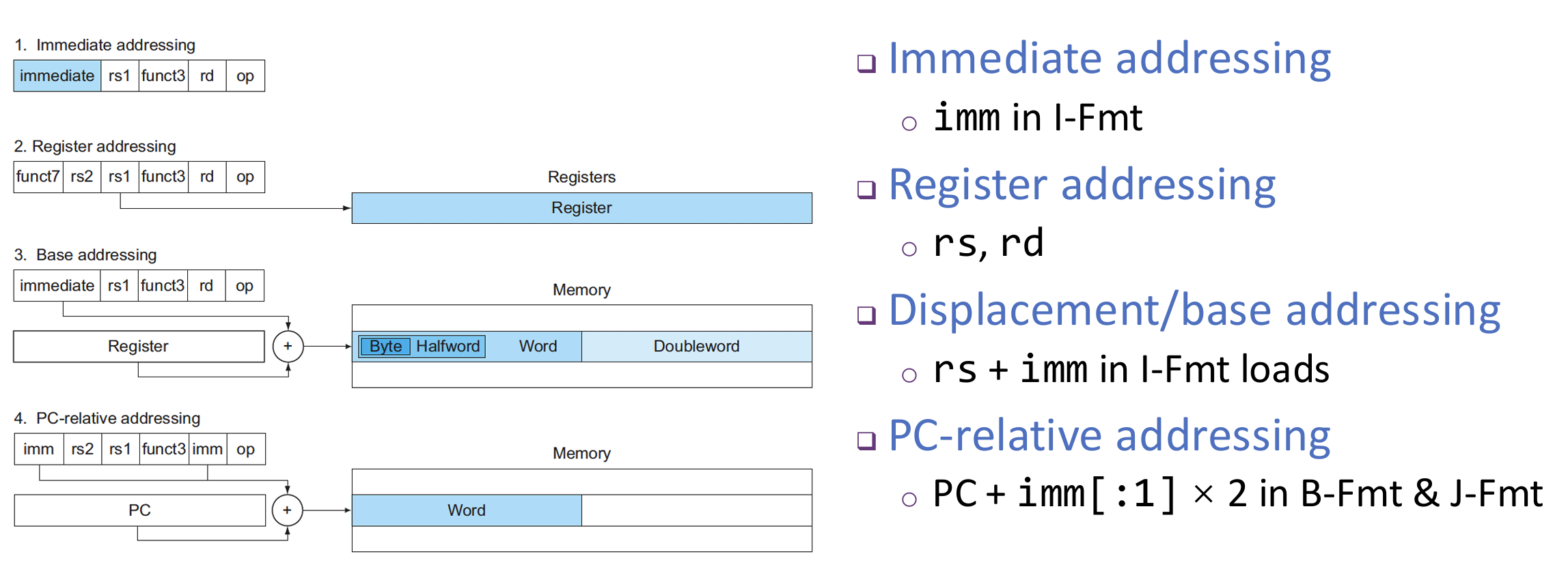
• lw rd, offset(rs1): Load a 32-bit word;
• sw rs2, offset(rs1): Store a 32-bit word.
• lh/lhu/sh: Load/store a halfword (16-bit), sign/zero-extend the loaded value
• lb/lbu/sb: Load/store a byte (8-bit). Addresses should be 4-aligned for lw/sw, 2-aligned for lh/sh, ...
• lui rd, imm: Load upper immediate, rd = imm (20-bit) | 0 (12-bit)
• auipc rd, imm: Add upper immediate to PC, rd = PC + (imm (20-bit) | 0 (12-bit))

Branch/Jump Instructions:

• beq/bne/blt/bge/bltu/bgeu rs1, rs2, L: Branch if equal/not equal/less than/not less than/less than unsigned/not less than unsigned
• jal rd, L: Jump and link. Store PC + 4 in rd; goto L
• jalr rd, rs1, offset: Jump and link register. Store PC + 4 in rd; goto rs1 + offset

If-else:

Switch-case:

While/for loops:

Procedure Calls and RISC-V Calling Convention

• Call: jump-and-link, jal ra, L
• Procedure arguments: Before calling via jal, caller stores the first 8 arguments in a0 to a7; others are passed through the stack.
• Return: jr ra
• Return values: Before returning via jr, callee stores the first 2 return values in a0, a1; others are passed through the stack.

The problem: both caller and callee would like to freely use registers; must save and restore register values before calling and after returning.

ISA clearly specifies caller/callee-saved registers.

• Caller-saved: caller saves before the call, and restores after the call returns. ra, t0 -- t6, a0 -- a7
• Callee-saved: callee saves before using, and restores before returning. sp, s0 -- s11 (fp is s0)

Stack Frame:

• sp (stack pointer): points to current stack top
• fp (frame pointer): points to current frame bottom

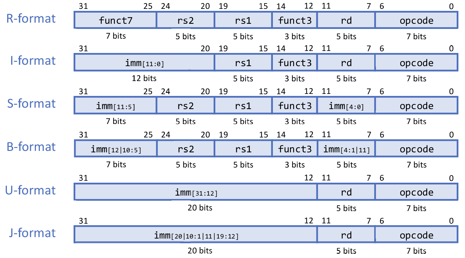
RISC-V Encoding

All instructions are 32-bit long and aligned in memory. There are six instruction formats:

• R-format: register-register operations
• I-format: register-immediate operations, loads, jalr (12-bit imm, 11:0)
• S-format: stores (12-bit imm, 11:0)
• B-format: branches (12-bit imm, 12:1)
• J-format: jumps (20-bit imm, 20:1)
• U-format: upper immediate instructions (20-bit imm, 31:12)

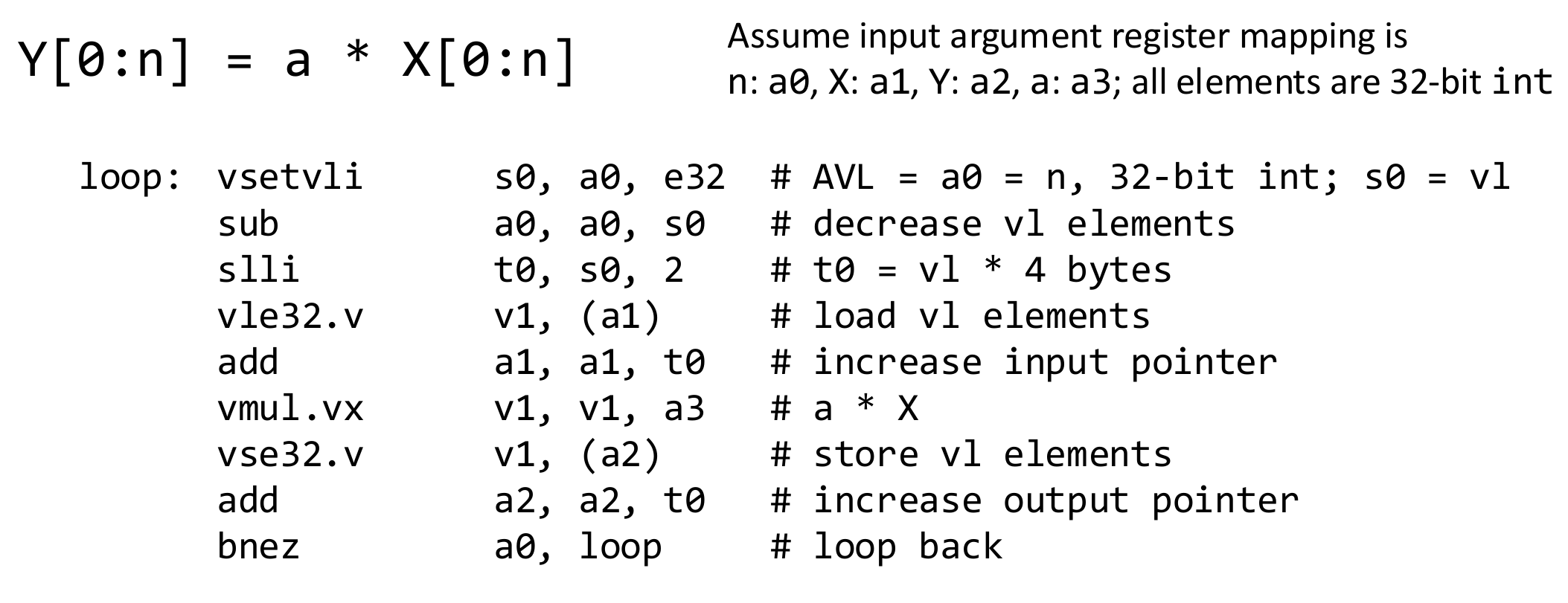
RISC-V Vector Extension

Single-Instruction, Multiple-Data. Compute on a vector of numbers simultaneously. Data-level parallelism.

Intel x86 SSE and AVX Extensions

Vector length keeps increasing.

Fixed total length can be split into various numbers of data types.

SIMD intrinsics: use C functions instead of inline assembly to call SSE/AVX instructions.

Function name: _mm<width>_[function]_[type]

A key drawback: vector length is hard-coded in instructions.

RISC-V Vector Extension

Similar to x86 SSE/AVX, use data-level parallelism, a.k.a., SIMD

Allow for variable vector length in software application.

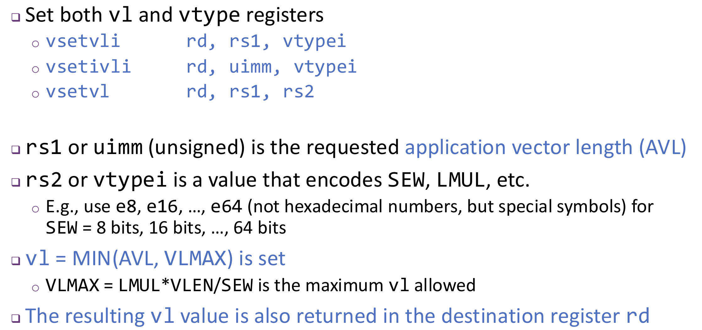
32 vector data registers: v0 to v31, each is VLEN bits long.

Vector length register vl: set the vector length in number of elements.

Vector configuration register vtype: LMUL, SEW, VLMAX, ...

• LMUL: vector register grouping multiplier
• SEW: selected element width

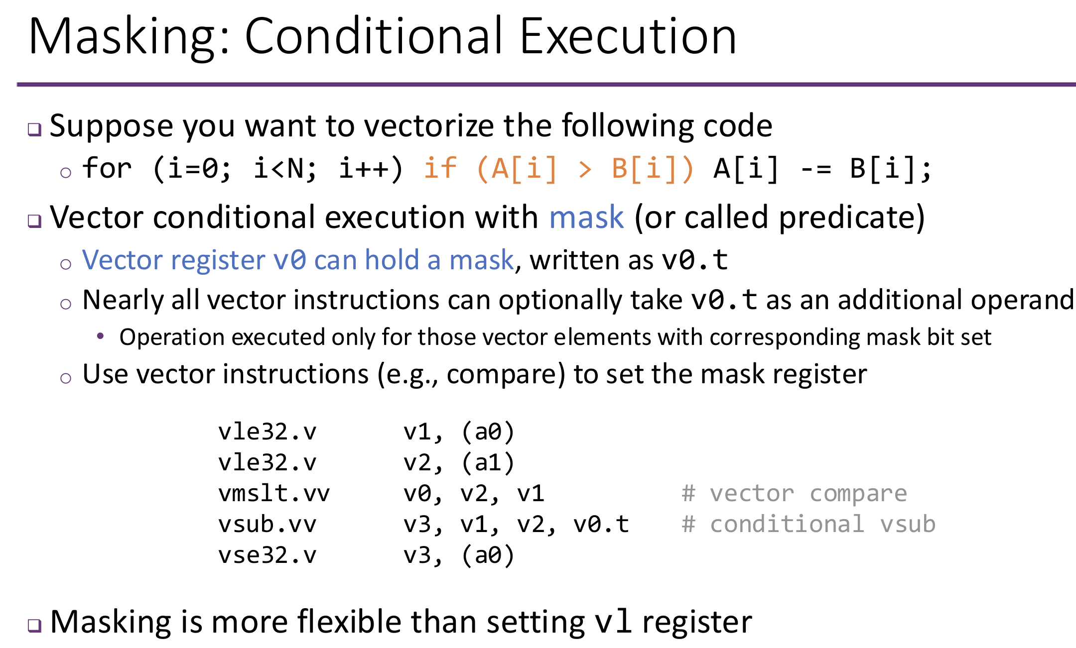
Advantages of Vector ISAs

• Compact: a single instruction defines N operations
• Parallel: N operations are (data) parallel
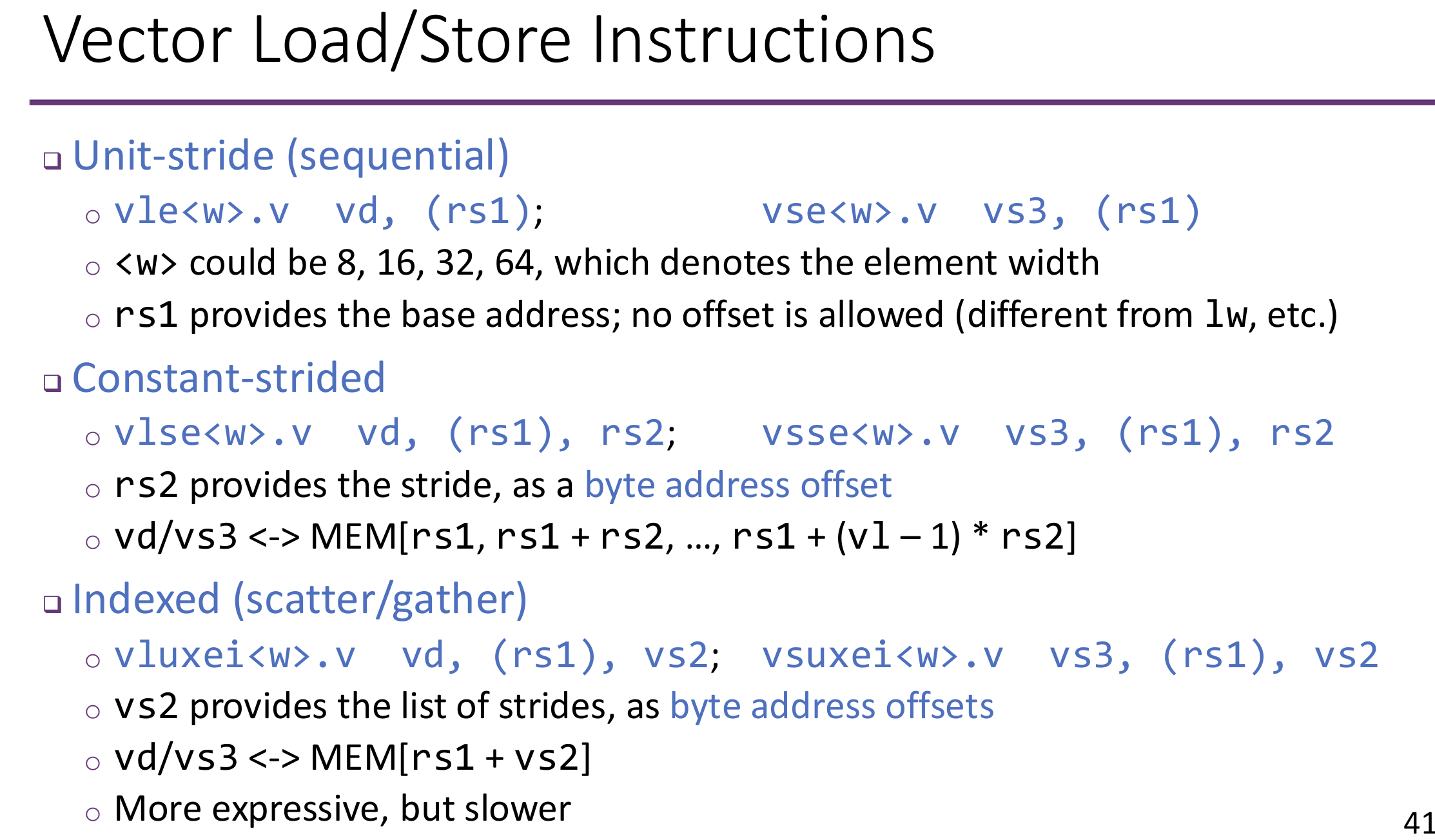
• Expressive: various memory patterns
• Compare to SSE/AVX: ISA is agnostic to hardware vector register length

Processor

Single-Cycle Processor

We will start simple, and later optimize for performance

• Execute one instruction to completion before moving to the next one
• Execute each instruction within one clock cycle, i.e., CPI = 1

We will focus on a subset of the RISC-V instructions

• Arithmetic (R, I): add, sub, addi, ori
• Memory (I, S): lw, sw
• Branch / jump (B, J): beq, j

Generally speaking, two parts:

• Datapath: the hardware that processes and stores data
• Control: the hardware that manages the datapath

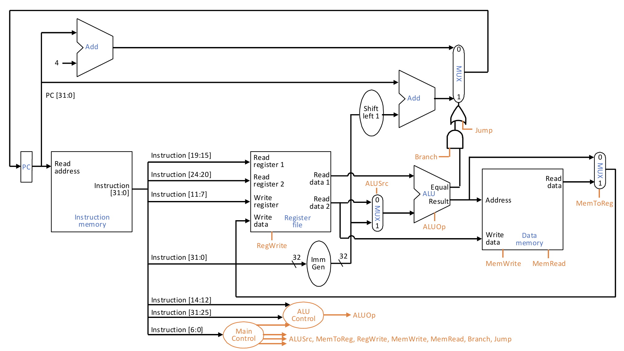
If we want update states one-after-one, CPI = 1, then the clock cycle time must be long enough to accommodate the slowest instruction.

Pipelined Processor

Basic Idea of Pipelining

For a \(k\)-stage pipeline,

\[f=\left(\frac{t_{\text{comb}}}{k}+t_{\text{reg}}\right)^{-1}. \]

Latency:

\[t_{\text{comb}}+ k \times t_{\text{reg}}. \]

Pipeline depth is limited by timing overhead of registers.

For \(N\) tasks of \(T\) time per task, \(k\) stage pipeline:

\[\frac{k-1}{k}T+\frac{N}{k}T. \]

In reality, combinational logic can not be equally divided, then pipeline throughput is limited by the slowest stage.

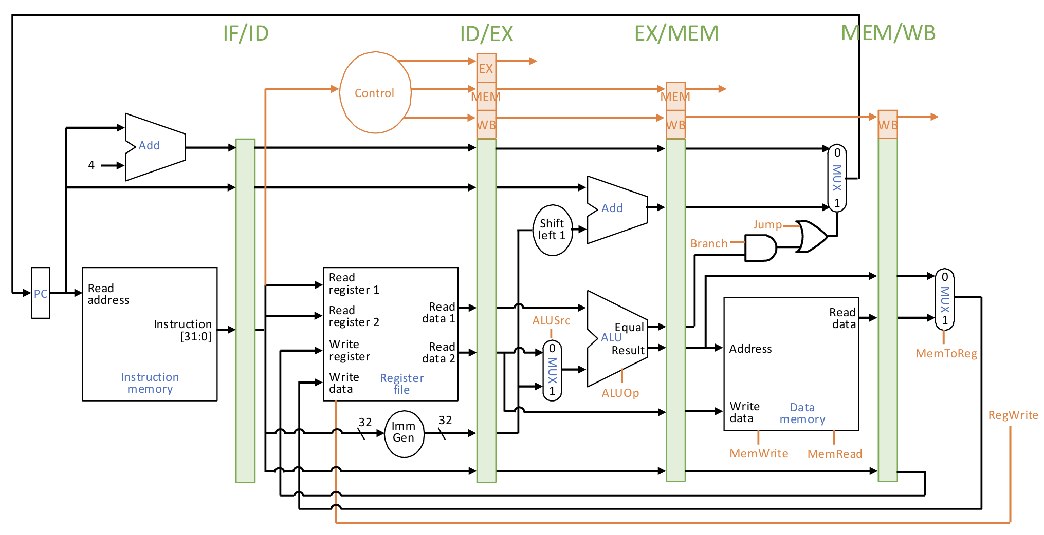
5-Stage Pipeline

5 stages, one clock cycle per stage

• IF (Instruction Fetch): fetch instruction from memory
• ID (Instruction Decode): decode instruction & read register
• EX (Execute): execute operation or calculate address
• MEM (Memory): access memory
• WB (Writeback): write result back to register

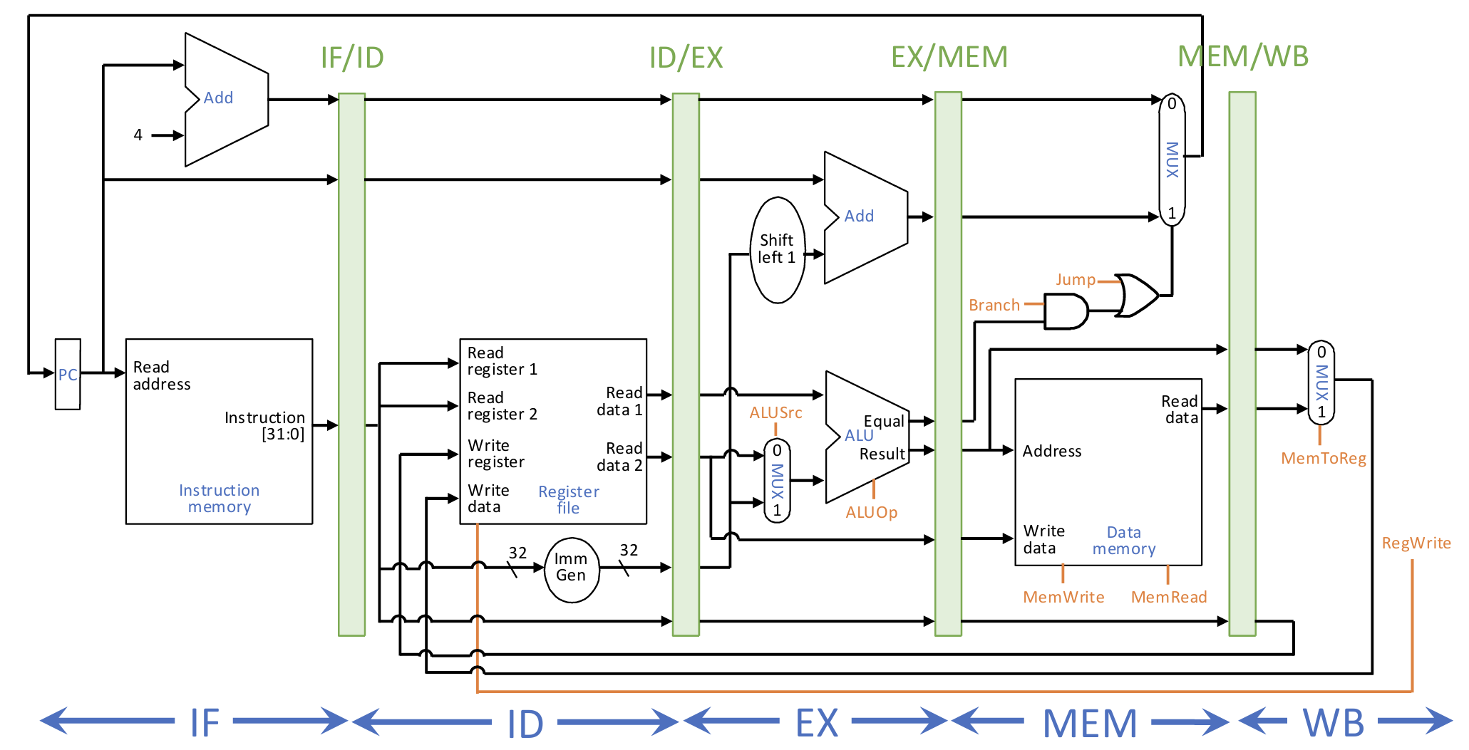
Pipelined Control Signals:

• Used 1 cycle later in EX: ALUOp, ALUSrc
• Used 2 cycles later in MEM: MemWrite, MemRead, Branch, Jump
• Used 3 cycles later in WB: MemToReg, RegWrite

Stalls and Hazards

Unfortunately, if two instructions are dependent, we encounter pipeline stalls. Stall is a pipeline “bubble”, not moving forward in that cycle.

Effective CPI = base CPI + stall cycles per instruction.

How to Stall:

• Software stalls: Compiler inserts independent instructions or nop instructions;
• Hardware stalls: Instructions before it continue to move forward as usual; prevent updates of PC and after registers.

Pipeline stalls are caused by hazards:

• Structural hazard: A required resource is busy and cannot be used in this cycle
• Data hazard: Must wait previous dependent instructions to produce/consume data
• Control hazard: Next PC depends on previous instruction

Structural hazard

Register File Access: A prior WB stage and a future ID stage both access registers

Solution: different read/write ports; half-cycle register access

Stage Bypassing: bypass unused stages, but cause structural hazard

Memory Access: Assume instruction & data memories are not separate, IF and MEM stages both access memory

Solution: replicate resources, i.e., use separate memories (caches), or use multiple ports

Multi-Cycle Instructions: instructions that are multi-cycle but not fully pipelined

Solution: make all units fully pipelined; replicate units; just let it stall

Data Hazard

Data Dependencies: Read after Write, Write after Write, Write after Read.

All dependencies must be respected, but pipelining may violate this promise.

In our 5-stage pipeline, only RAW hazards through registers exist.

Solution: Stall pipeline to delay reading instructions until data are available.

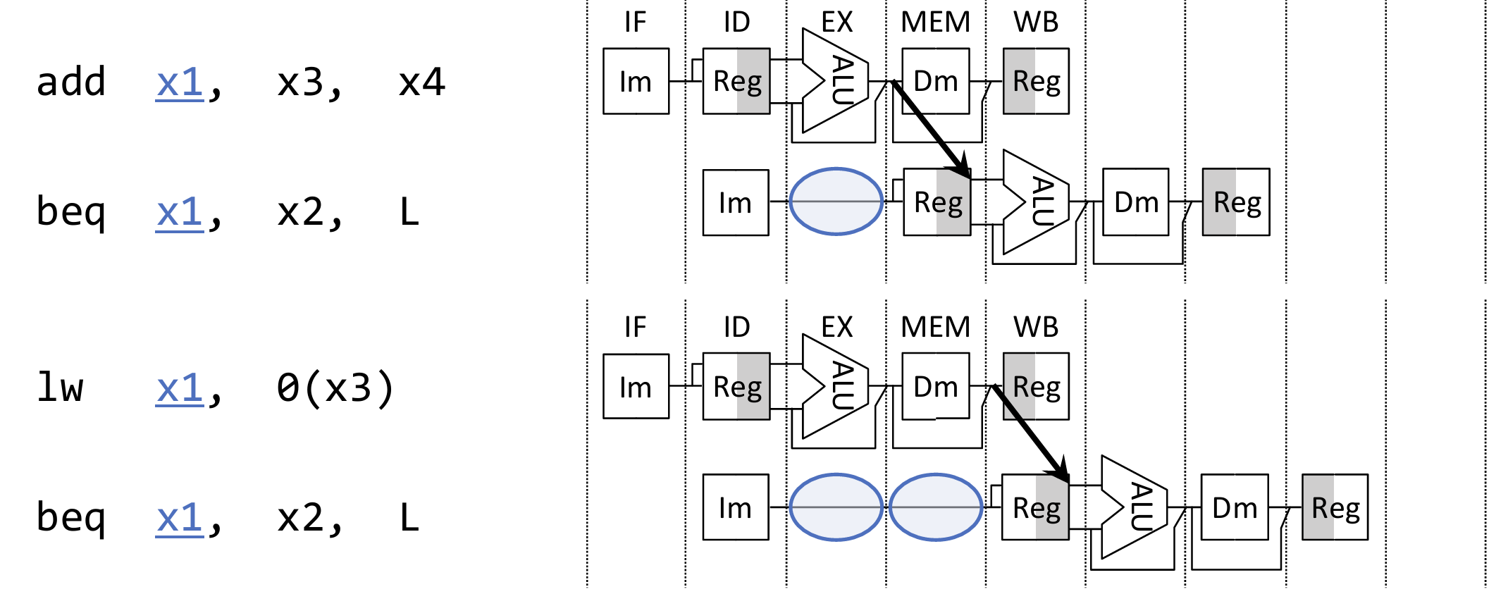
A better way is to use Data Forwarding (bypassing): Adding additional hardware paths, the calculation results are "forwarded" directly from where they are generated to the subsequent instructions that need them, thus avoiding pipeline stalls.

How many remaining cycles to stall after forwarding is corresponding to the stage distance between producer and consumer. In our 5-stage pipeline, only load-use hazard needs to stall 1 cycle.

Forwarding Datapath:

• Destinations: all stages that really consume values: EX, MEM
• Sources: stages after all stages that produce new values: MEM, WB
• We let forwarding sources from the pipeline registers

Forwarding Control:

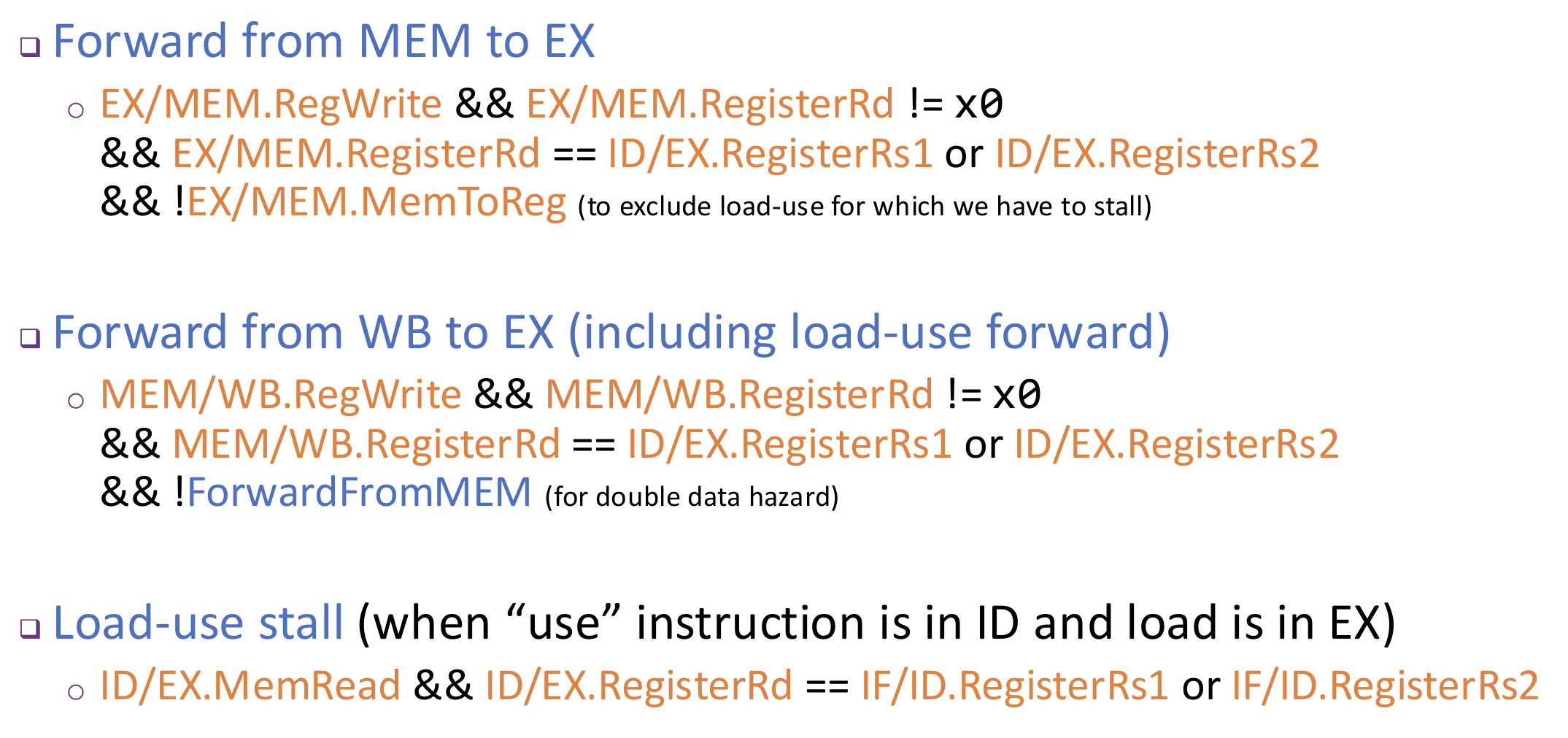
Whole picture:

Compilers can rearrange code to avoid load-use stalls, a.k.a., to fill the load delay slot.

Control Hazard

Cannot fetch the next instruction if I don’t know its address (PC).

Possible next PC in RISC-V

• Most instructions: PC + 4 (Calculated in IF stage)
• Jumps: PC + offset
• Branches: PC+ 4 or PC + offset, after comparing registers

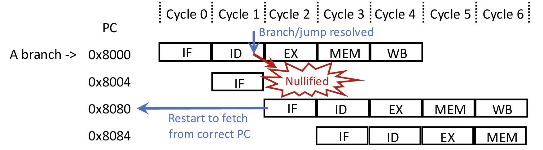
To resolve branch/jump target early, we can moved the branch/jump resolving point to ID stage.

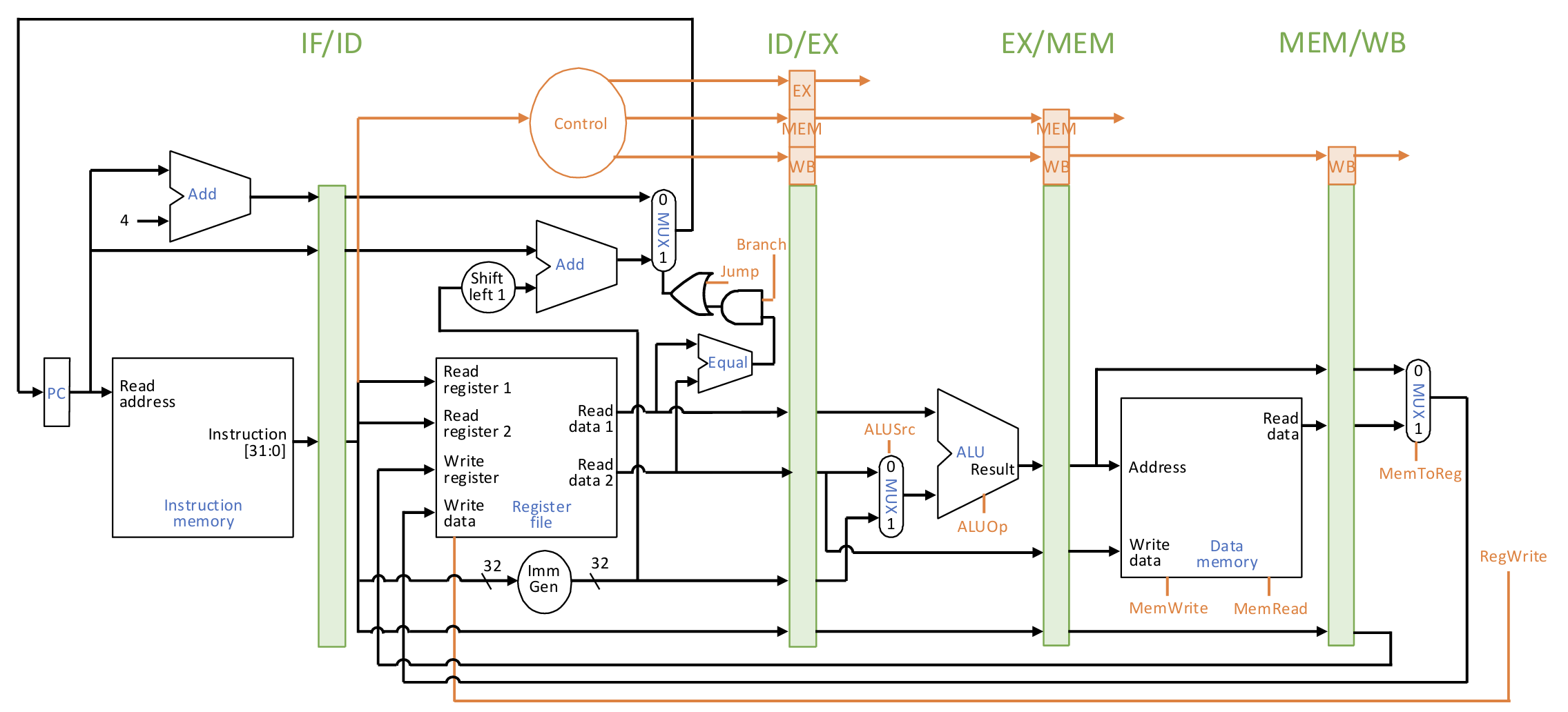
Now we only need to 1-cycle stall for next PC. Furthermore, we can simply guess that next PC is PC + 4, and if the guess is wrong, flush pipeline to nullify mispredicted instructions. Restart wastes 1 cycle + some extra penalty cycles.

Additional forwarding paths of register values to ID stage: 1-cycle stall for previous ALU operation, 2-cycle stall for previous load.

Exceptions and Interrupts

So far two ways to change control flow within user programs

• Branch and jump
• Call and return

Insufficient for changes in system states

• Exception: internal "unexcepted" events in the program itself
• Interrupts: external events (e.g., I/O) that require processor handling

User programs cannot anticipate or always prepare for these events; require helps from the OS and the hardware.

OS, i.e., the privileged kernel, handles exceptions/interrupts

• Processor stops the user program, saves current PC and the cause, and transfers
  control flow to the kernel
• Exceptions/interrupts are processed by exception handler inside the kernel, to fix problems or handle events
• Return to user program to continue (the current instruction or the next instruction); or abort if problems cannot be fixed

Handling Exceptions in RISC-V:

• Save PC (SEPC)
• Save the reason (SCAUSE)
• Jump to the handler at a fixed address in kernel, e.g., 0x80000000
• The handler reads the cause register to decide what to do:
  • If fixable, take corrective actions and use SEPC to return to user code
  • Otherwise, terminate program and report error using SEPC and SCAUSE

Alternate Mechanism: Vectored Interrupts (used in x86): separate handlers for different causes

Requirements of precise exceptions:

• All previous instructions had completed
• None of the offending instruction and the following instructions were started

All in all, when exception/interrupt occurs in the pipeline:

• Drain older instructions down the pipeline to complete
• Nullify the current and younger instructions in earlier stages
• Fetch from handler instruction address

Advanced Techniques

Branch Prediction

We need more powerful branch prediction! Two steps:

• Predict a branch is taken or not-taken;
• Predict the target address if taken.

Remember, with either result, after resolving the branch, if mispredicted, flush and restart.

To predict taken/not-taken, besides exploiting hints from programmers/compilers, we can do hardware-based dynamic prediction, i.e., based on recent history.

A hardware branch history table (BHT) records each branch's history. It only use \(m\) bits of the PC to index. Each branch maintains a saturate counter that summarizes the history, which is used to predict the next direction.

• Counter +1 for an actually taken branch (until max),–1 for not-taken (until min)
• 1-bit states: 0: predict not-taken, 1: predict taken
• 2-bit states: 00: predict not-taken, 01: not-taken?, 10: taken?, 11: taken

Essentially a tradeoff between robustness and adaptivity.

To predict target address, we can use a branch target buffer (BTB) that caches the target addresses of recently taken branches. Note that here we also store the rest of the address as a tag to differentiate aliasing cases.

Superscalar and Out-of-Order

Let \(T_1\) be the time to execute with one compute unit, and \(T_\infty\) be the time to execute with infinite compute units. Instruction-Level Parallelism:$$\text{ILP} =\frac{T_1}{T_\infty}$$ measures inter-(in)dependency among instructions.

Scalar pipelines are limited by \(\text{IPC}_\text{max} = 1\), while superscalar pipelines can issue at most \(\text{IPC}_\text{max} = N\) for \(N\)-way superscalar. To implement superscalar, we need out-of-order (OoO) execution:

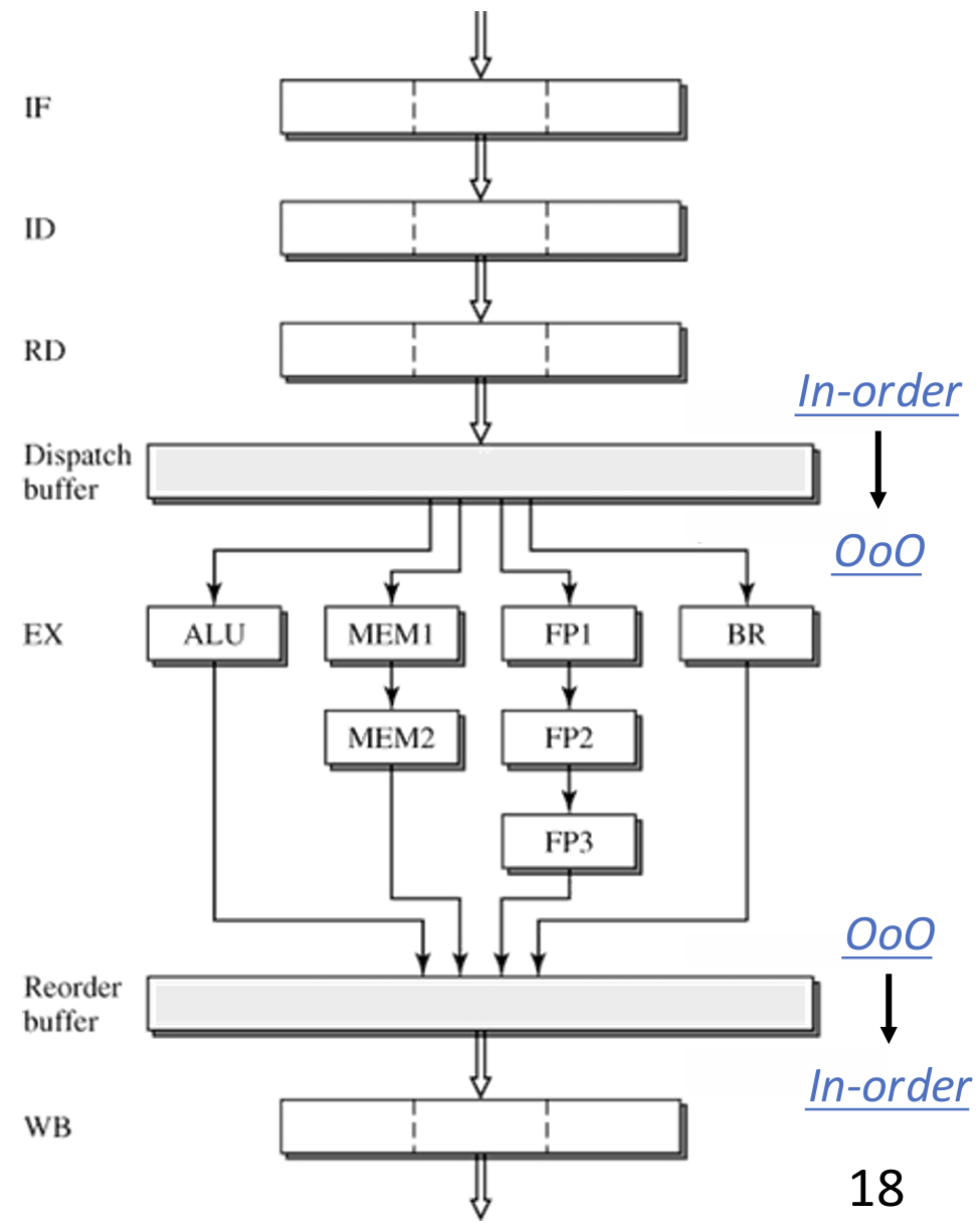
Stages:

• Fetch: wide and speculative
• Decode
• Dispatch/rename/allocation: must be in-order
• Issue/schedule: Instruction window (IW) to store the data between dispatch and execute, and scheduler decides which instruction to issue based on its priority.
• Execute
• Reorder: Re-Order Buffer (ROB): a FIFO for instruction tracking
• Commit/retire/write-back: must be in-order. Instructions that finish execution but have not commit are considered speculative, and hold their updates to system states. Check the head of ROB in each cycle.

Limitations of Modern Processors

Limitations:

• Limited ILP in programs
• Pipelining overheads
• Frontend bottleneck
• Memory inefficiency
• Implementation complexity

Solutions:

• Parallelism: multi-core
• Better design: ASIC (application-specific integrated circuits)

Still, we have data access challenge: when processors get improved, memory performance and energy start to dominate

Memory

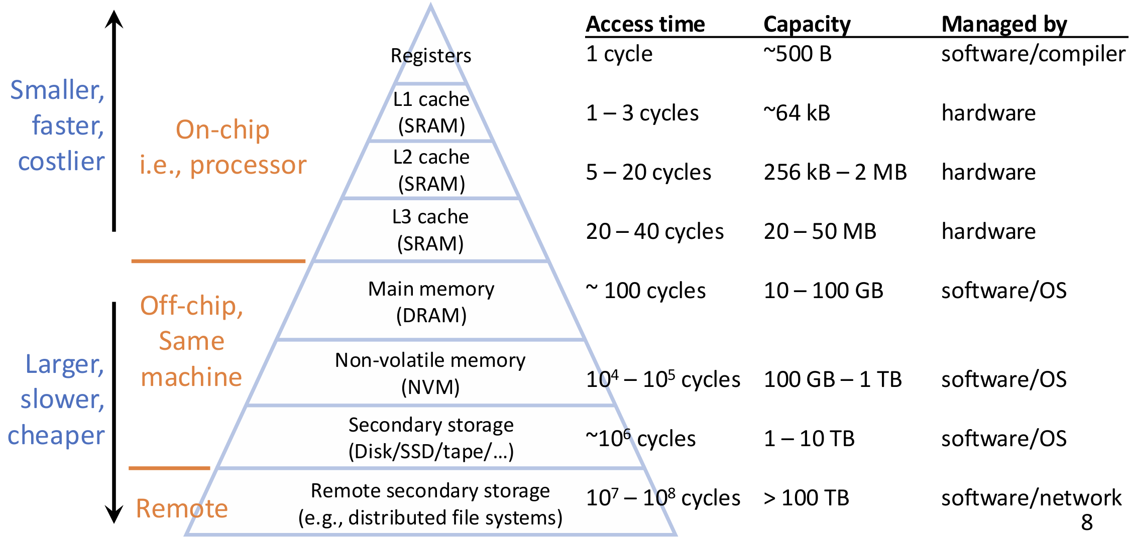
Memory Hierarchy: the faster, smaller device at level \(k\) store a subset of data for the larger, slower device at level \(k+1\).

Caches

Caches are implemented as processor components, which hold recently referenced data by exploiting locality. Managed by hardware, and invisible to software.

In cache, data is transferred in unit of blocks, a.k.a., cachelines.

• Cache hit: data found in the cache; serve with short latency
• Cache miss: data not found in the cache; need to fetch the block from memory, and may replace a block in the cache

AMAT (average memory access time) = hit latency + miss rate \(\times\) miss penalty

Cache Organization

Fully Associative: a block can be put anywhere in the cache.

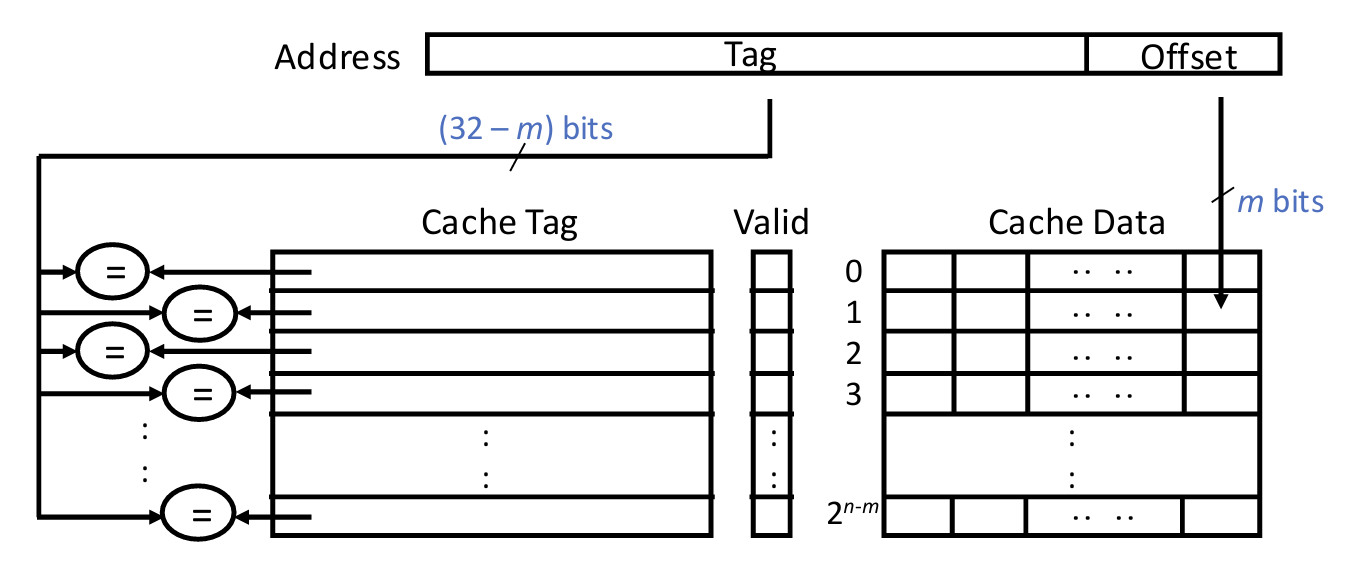
• Pros: have the maximum utilization to cache data, i.e., low miss rate
• Cons: slow to look up a block(must look at every location), i.e., high hit latency

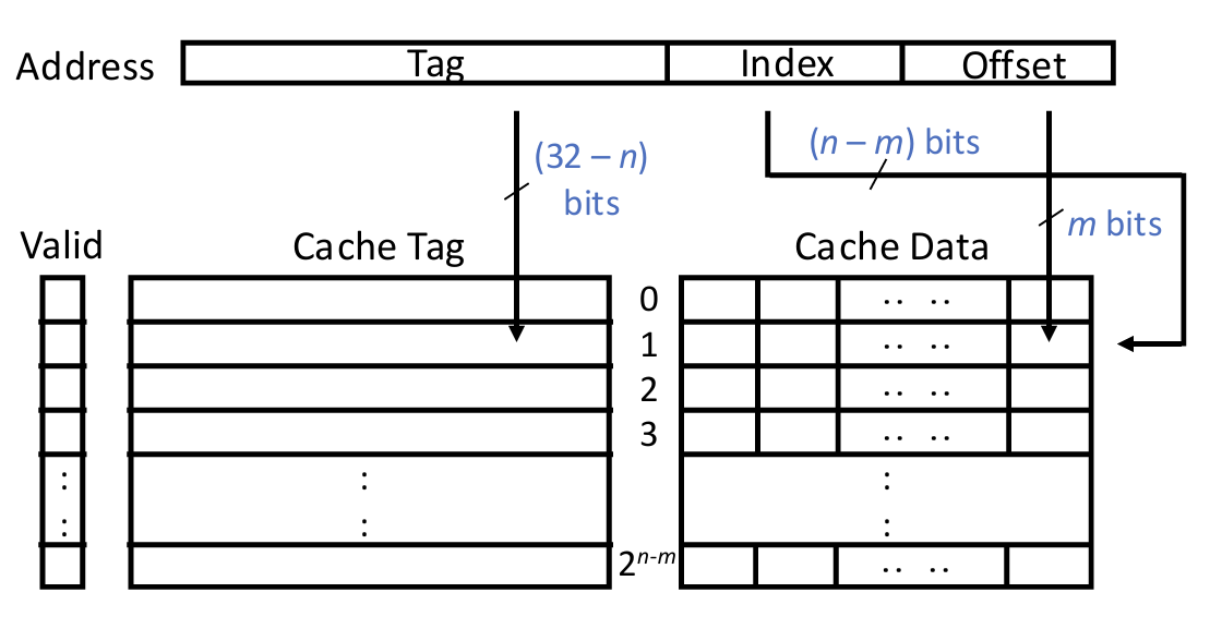
Direct-Mapped: each block has only one determined location, according to its memory address.

• Pros: fast to lookup, i.e., low hit latency
• Cons: more conflicts between blocks, i.e., high miss rate

Set-Associative (\(N\)-way): each block can go to one of \(N\) entries in cache.

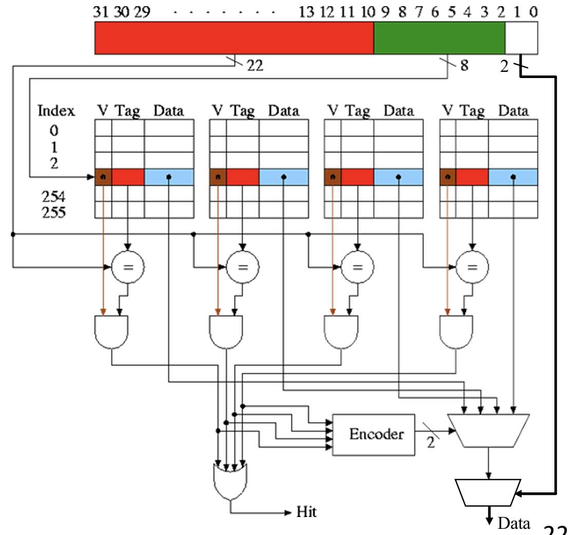
Cache access steps:

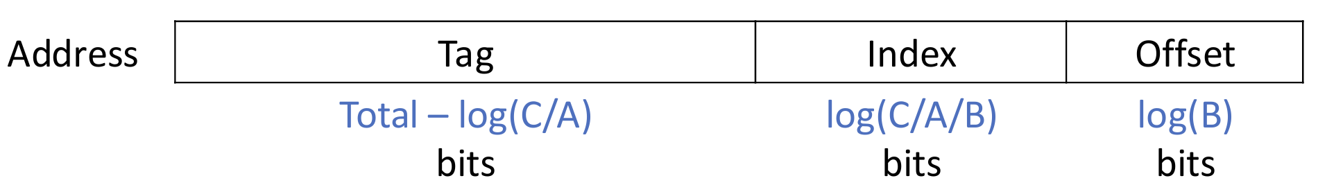
• Decompose address bits into tag, index, offset
• Use index bits to locate a set
• For each entry in the set
  • Check if valid bit is 1
  • Compare if tag matches
• If found one such entry, hit, return data
  • Useoffset to select bytes in block
• If none found, miss, fetch data from memory, return data, and replace

The 3Cs of Cache Misses

• Compulsory/cold: the first time the item is referenced
• Capacity: not enough room in the cache to hold all items
• Conflict: item is replaced because of a location conflict with others

Design configurations:

• Capacity: capacity misses
  • Thrashing: scan data for multiple times, but cache capacity is insufficient
  • Solution: optimize code to fully work on each subset before the next
• Associativity: conflict misses
  • Conflicts could happen quite often in real programs
  • Solution: use more complex hashfunctions to determine set index
• Block Size: compulsory misses

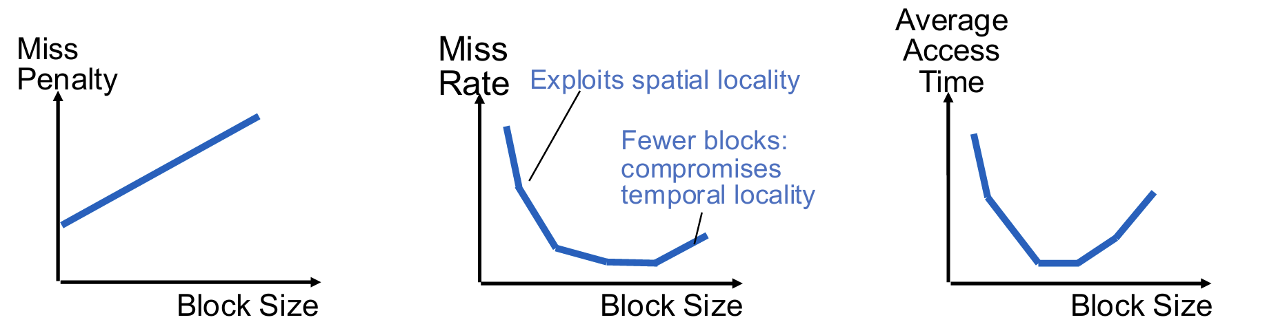
For the address fields

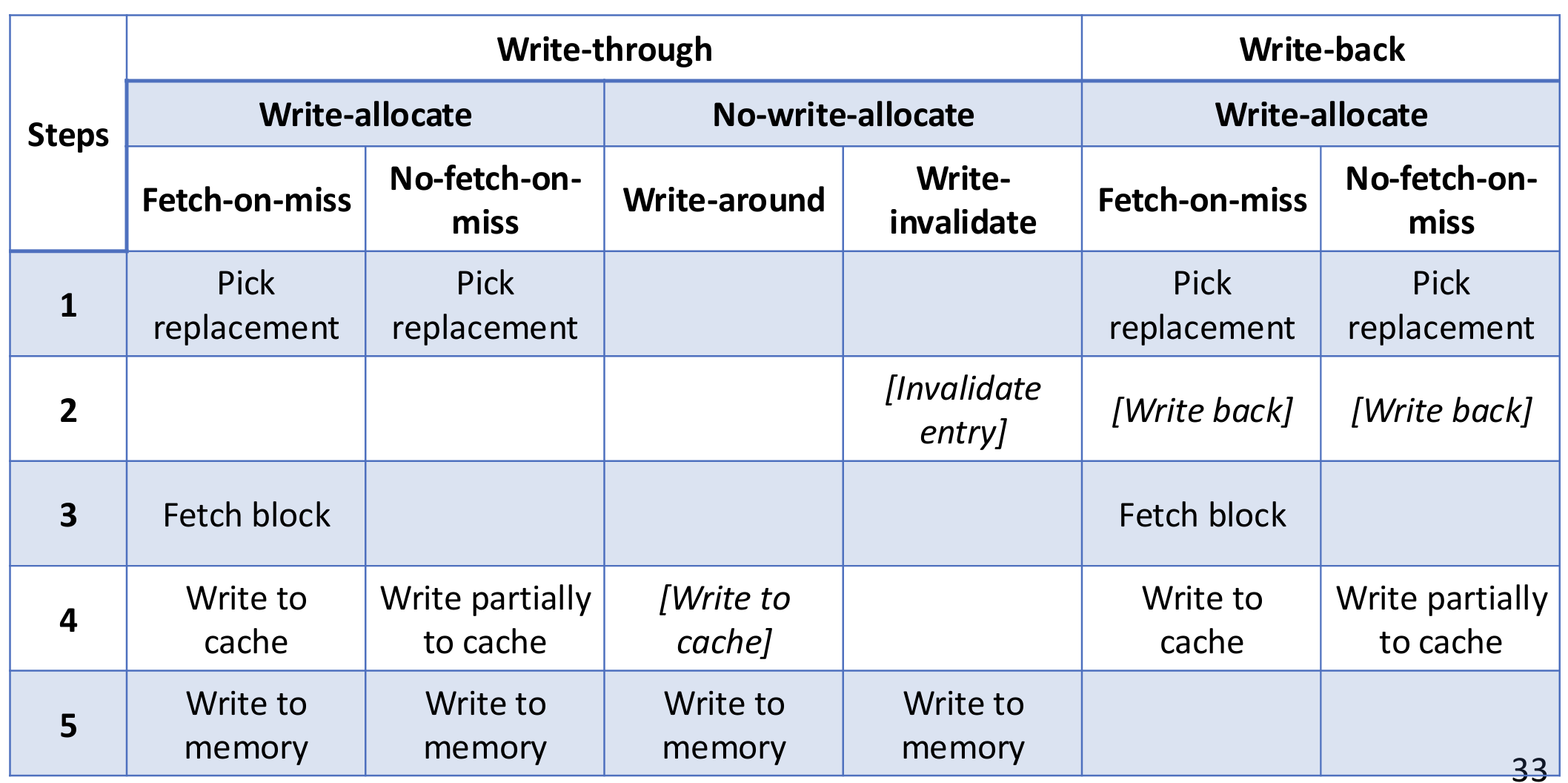
Write Policies

Write misses are less performance critical than read misses.

Write Hits:

• Write-through: update both cache and memory
• Write-back: write data only to cache

Write Misses:

• Write-allocate: load the block into cache, then write
  • Fetch-on-miss or not: do we fetch the rest of the block from memory?
• No-write-allocate: bypass cache, write directly to memory
  • Write-around vs. write-invalidate: do we keep the data in cache if there is already an entry (e.g., due to reads)?

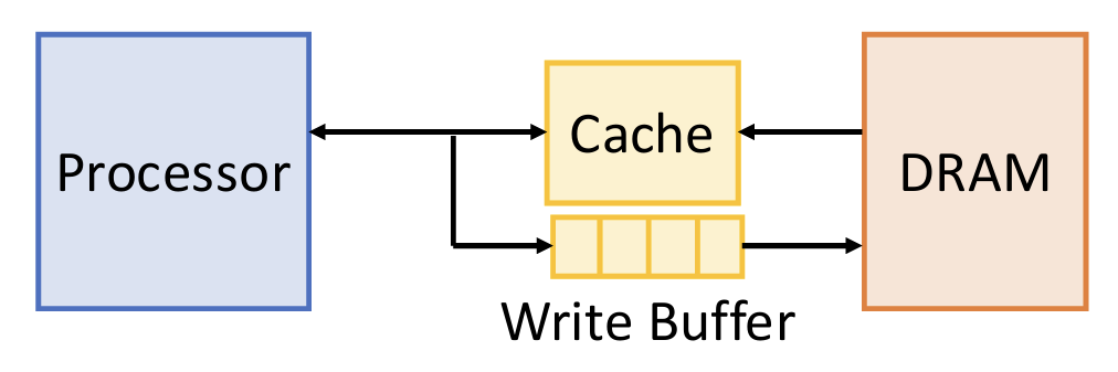
For write-through, we use write buffer, a FIFO buffer between cache and memory. Can absorb small bursts, as long as the long-term rate of writing to the buffer does not exceed the maximum rate of writing to memory.

Typical Choices for Cache Write Policies:

• Write-back + write-allocate + fetch-on-miss

Replacement Policies

On a miss, determine whether to evict an existing entry to make room for the newly requested block, and if so, which entry to evict (called victim).

Whether to evict

• Normal: newly requested block replaces an existing old block
• Bypass: newly requested block does not enter cache

Which to evict

• For direct-mapped, only one choice
• For set/fully associative, use a replacement policy

Replacement policy virtually keeps a rank (a priority list) of cache blocks. To define a new policy, we need to define insertion policy (when a block is first inserted into cache) and promotion policy (when an access hit on the block in cache). Priority from MRU to LRU.

Recency-Based Policies:

• LRU (Least Recently Used): insert/promote to MRU
• LIP (LRU insertion policy): insert to LRU, promote to MRU
• BIP (Bimodal insertion policy): combine LRU and LIP, insert with small probability at MRU, others at LRU
• DIP (Dynamic Insertion Policy): dynamically select between LRU and BIP

How to implement DIP? A simple way is to use shadow/ghost tag arrays: maintain two tag arrays for LRU and BIP, respectively, to track their miss rates. Use the one with lower miss rate for actual cache replacement.

Another way is to use set dueling: dedicate some sets to different policies, and select the best performing one for the rest sets.

Frequency-Based Policies:

• LFU (Least Frequently Used): choose the one used the least

  • LFU adapts poorly to pattern changes. Let's combine recency and frequency.

• FBR (frequency-based replacement): Do not increment counters for recently referenced (i.e., high-locality) blocks

• LRFU (least recently/frequently used): Accumulate a weighted value \(F(x)\) for each past reference, \(x\) is the distance from that reference to current time

Other Policies:

• Random: choose one at random; not necessarily a bad policy
• Belady's optimal: choose the one used again furthest in the future

Multi-Level Caches

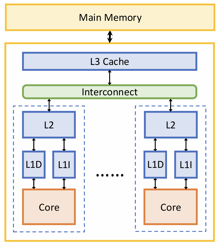
• L1 caches attached to CPU cores. Split D-cache & I-cache (D & I). Focus on hit time.
• L2 unified cache per core
• L3 cache is shared across all cores, a.k.a., last-level cache (LLC). Focus on miss rate.

Inclusion

Inclusive caches: data in this level are always a subset of data in parent

• Advantages: Only check the last level to know if a block is not cached in the entire hierarchy; Writeback is easy, eviction from children always hits in parent
• Disadvantages: Data are replicated in both cache levels, lower utilization; Eviction in parent must also evict the block in children, a.k.a., recall

Exclusive caches: data in this level are NOT ALLOWED in parent

Non-inclusive caches: data in this level may be in parent

• Save cache space, potentially higher hit rates: better performance
• Significantly complicate management

Performance

AMAT for Multi-Level Caches
= L1 hit latency + L1 miss rate × AMAT ofL 2
= L1 hit latency + L1 miss rate × (L2 hit latency + L2 miss rate × AMAT of L3)
= ...

Local miss rate = # misses in this level / # accesses to this level

Global miss rate = # misses in this level / # accesses from processor.

So AMAT = L1 hit latency + L1 global miss rate × L2 hit latency + L2 global miss rate × L3 hit latency + ...

Overall, multi-level caches achieve good balance between miss rate and hit time, i.e., a smoothly, gradually changing spectrum of capacity vs. access speed, to capture different degrees of locality and dataset sizes.

Non-Blocking Caches

Cache needs to support multiple accesses

• Allow for hits while serving a miss (hit-under-miss)
• Allow for hits to pending misses (hit-to-miss) to avoid redundant memory fetches
• Allow for more than one outstanding miss (miss-under-miss)

Miss Status Handling Register (MSHR) keeps track of each outstanding miss to one cache block, as well as pending loads & stores that refer to that block

• Multiple misses to different blocks are tracked in different MSHRs
• Multiple loads/stores to the same block are in one MSHR

Fields of an MSHR: valid bit, block address and multiple pending load/store entries.

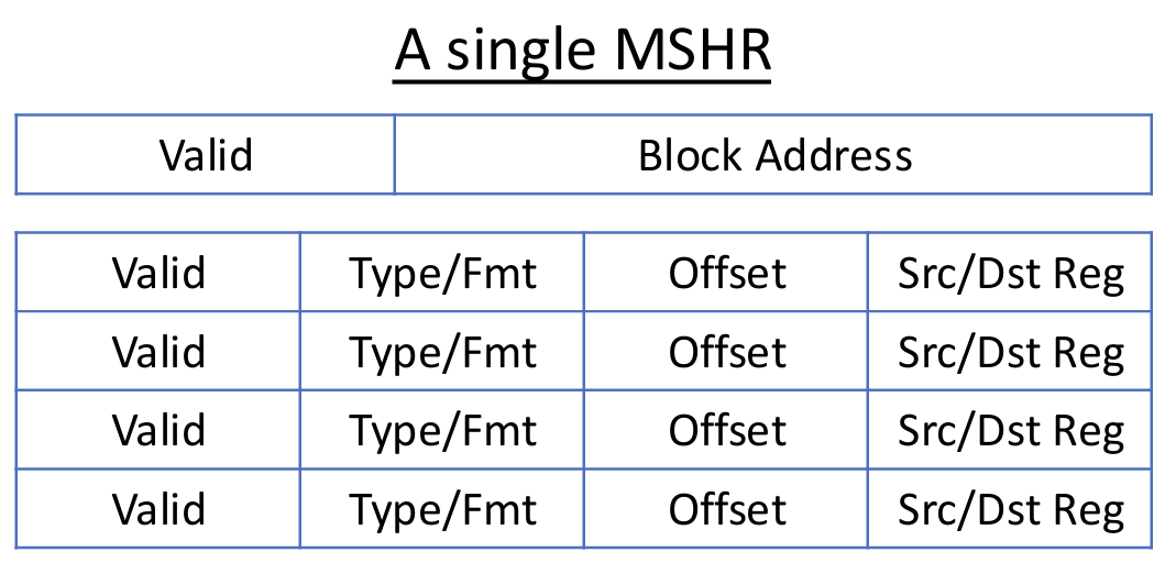
Operations:

• On a cache miss
  • Search MSHRs for pending access to this cache block
  • If found, just allocate a new load/store entry in that MSHR (hit-to-miss)
  • Otherwise allocate a new MSHR and its first load/store entry (miss-under-miss)
  • If no MSHR or load/store entry free, stall
• By offloading states to MSHR, cache can process other requests
• When one word/sub-block of a cache block becomes available
  • Check which loads/stores are waiting for it, and forward data to/from core
  • Clear the load/store entry
• When last word of a cache block becomes available
  • All load/store entries of this MSHR can be served
  • Clear MSHR

Data Prefetching

We want to predict and fetch data into cache before processors request it, so that we can reduce cold misses by exploiting spatial locality. Must have non-blocking caches!

Software prefetch instructions, e.g., GCC __builtin_prefetch() are micro-architecture-dependent, while hardware prefetchers are automatic.

Metrics:

• Accuracy = (prefetched & accessed) / (all prefetched)
• Coverage = (prefetched & accessed) / (all accessed)

Timeliness: you issue prefetch requests early enough, but not too early

Resource contention: prefetching consumes bandwidth and capacity

Types of Hardware Prefetchers:

• Stream Prefetching: prefetch N blocks ahead of the current access, only when detecting stream access patterns
• Strided Prefetching: detect strided access patterns and prefetch accordingly
  • PC-based stride detection: maintain a table indexed by PC, each entry records the last address and the stride.
• Temporal Correlation: learn the transition probabilities between cache blocks, and prefetch according to the most probable next blocks.
• Spatial Correlation: learn the spatial patterns of accesses, and prefetch the correlated blocks together.

Main Memory

DRAM Organization

Main memory is physically separate from the processor chip (remember caches are on-chip), connected through memory channels.

DRAM is the prominent technology for main memory today. Key design goal of DRAM: use high bandwidth to tolerate long latency.

Organization of DRAM-based main memory:

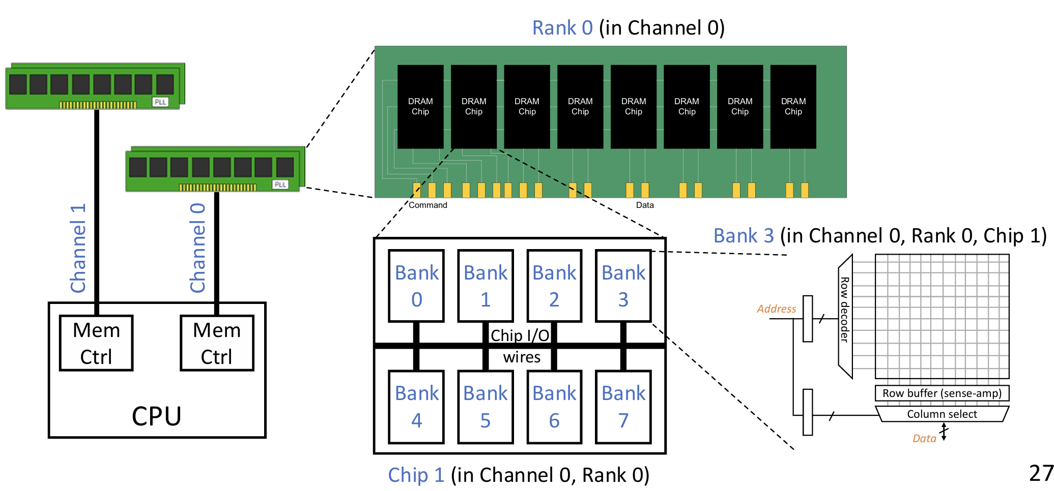
• Multiple channels per CPU socket: fully independent access with separate physical links (channel bus)
• Multiple ranks per channel: independent access inside chips, but share I/O (channel bus)
• Multiple chips per rank: fully synchronous access across all chips in a rank
• Multiple banks per chip: independent access inside banks, but share I/O (chip pins and internal bus)

Access granularity

• Each access needs multiple bytes; usually goes to a single <channel, rank, bank>
• The same bank in all chips of a rank contributes a subset of data
• The bytes are transferred on the bus sequentially in multiple cycles

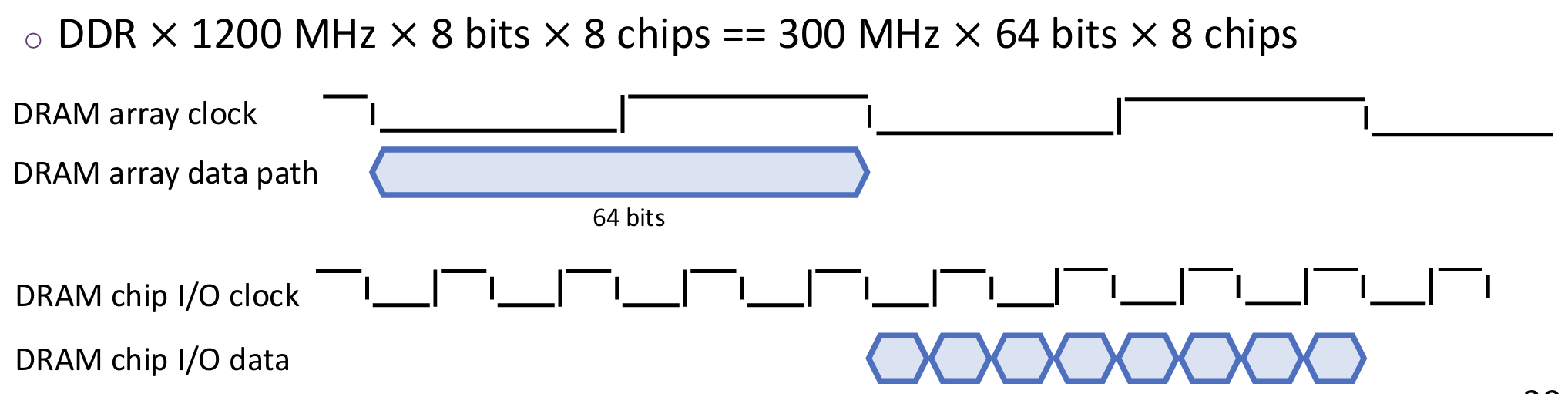
Channel:

• Each 64-byte access needs 8 burst transfers in 4 cycles on 64-bit channel bus. DDR: double-data-rate, i.e., transfer on both clock edges, e.g., 400 MHz == 800 MT/s.
• Channel-level parallelism: higher bandwidth and capacity. NUMA: non-uniform memory access, i.e., different channels have different access latencies.

Rank:

• Each access goes to one rank, selected using "Chip Select" signal. 64-bit data across all chips in a rank
• Ranks are physically organized in DIMMs
• Rank-level parallelism: Larger capacity
• Multiple narrow-I/O chips are put together for a wide rank interface

Ranks vs. Banks vs. Chips

• Banks and ranks are similar. They divide DRAM into multiple independent parts, allowing for overlapped accesses. The difference is just across vs. within chips。
• Chips are to make I/O width wider. Purely a physical organization, without affecting logical hierarchy.

Inside a DRAM bank, data are stored in rows and columns. Each row corresponds to a wordline, and each column corresponds to \(w\) bitlines, where \(w\) is the I/O width of the DRAM chip.

Access sequence:

1. Decode row address & drive wordlines
2. Selected cell bits drive bitlines
3. Entire row read into row buffer and amplify
4. Decode column address & select columns
5. Precharge bitlines for next access

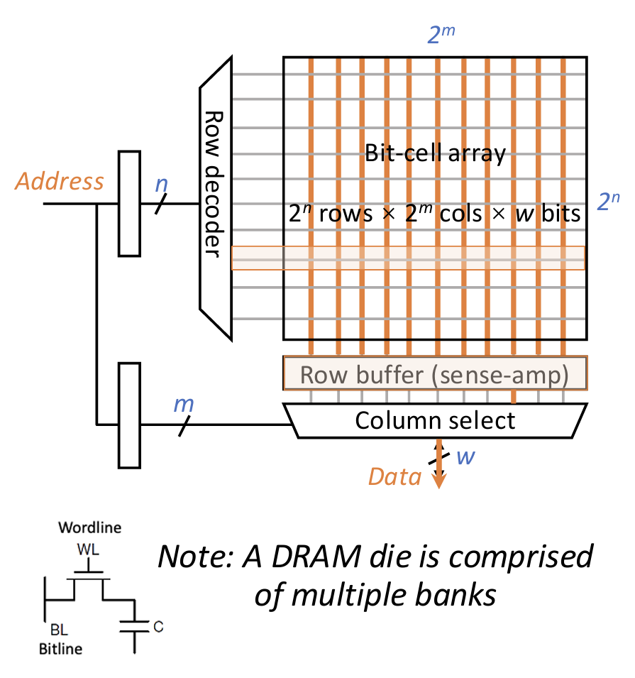
5 basic commands

• ACTIVATE (open a row)
• READ (read columns in a burst)
• WRITE (write columns in a burst)
• PRECHARGE (close the row)
• REFRESH

Overfetch: Accessing one cell must first activate the entire row to row buffer

• Benefit: reduced area overheads of row/column logic w.r.t. dense cell arrays
• Downside: higher latency and energy; but can amortize if there is good locality

Row hits save latency and energy, while row conflicts incur extra latency and energy overheads.

DRAM I/O is clocked faster than DRAM arrays, while internal access from arrays is wider than I/O width.

Overview of Parallelism:

• Multiple channels per CPU socket: Support fully concurrent access, separate address/command/data
• Multiple ranks per channel: Support overlapped access, but share address/command/data
• Multiple chips per rank: Support lock-step access, share address/command, separate data
• Multiple banks per chip: Support overlapped access, but share address/command/data

IO 64B = 8 bursts × 8 chips × 8 bits (array width)

DRAM Management

Memory Controller (MC) manages DRAM access from (inside) processors. Functionality:

• Translate commands: loads/stores → ACTIVATE/READ/WRITE/PRECHARGE/…
• Enforce access timing constraints
• Decide address mapping: address → (channel, bank, row, col, …)
• Schedule access requests and manage row buffers
• Manage DRAM refresh
• Manage power modes, e.g., entering low-power

Latency of DRAM access:

1. CPU → memory controller transfer time
2. Controller latency
   • Convert to basic commands, queuing & scheduling delay
3. DRAM bank latency
   • Hit an openrow: tCAS, i.e., RD/WR
     • tCAS = time of column access strobe
   • Access an close row and row buffer empty: tRCD + tCAS, i.e., ACT + RD/WR
     • tRCD = row to column command delay
   • Access a conflict row from row buffer: tRP + tRCD + tCAS, i.e., PRE + ACT + RD/WR
     • tRP = time to precharge DRAM array
4. DRAM data transfer time = channel width * burst length / bandwidth
5. Memory controller → CPU transfer time

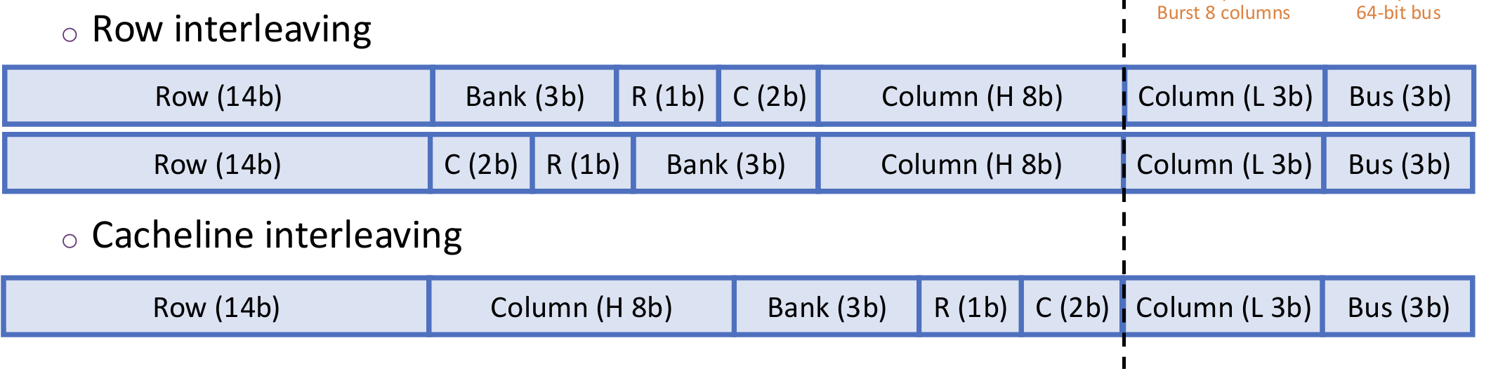
Physical address are mapped to <channel x, rank y, bank z, row r, column c>

For sequential accesses, we want to maximize row hits and bank-level parallelism. So cacheline interleaving is preferred. For strided accesses, row interleaving is better.

Row Buffer policies:

• Open-page policy: Expect next access to hit, leave row open after access (do not PRECHARGE)
  • Pros: if next access is a row hit, no need to ACTIVATE
  • Cons: if next access is not a row hit, extra latency to PRECHARGE
• Closed-page policy: Expect next access to conflict, immediately PRECHARGE
  • Pros: if next access is a row conflict, save PRECHARGE latency
  • Cons: if next access is a row hit, waste PRECHARGE/ACTIVATE latency and energy
• Adaptive policy: predict whether next access will hit or not

Scheduling Policies:

• FCFS (first come, first served)
• FR-FCFS (first ready, first come, first served)
  • Row-hit first, then oldest first
  • Goal: maximize row buffer hits

DRAM cell capacitor charge leaks over time, need to touch each cell periodically to restore the charge. So Refresh = ACTIVATE + PRECHARGE each row every N (64ms typically) milliseconds.

Between Cache and Main Memory

Cache Coherence

Copies of shared data in private caches can become stale & incoherent! We need cache coherence protocols to ensure that all caches have a consistent view of memory.

Basic rule of coherence: single-writer, multiple-readers (SWMR)

• All caches can have copies of data while read-shared
• On a write, invalidate all other copies, and leave a single writer

A 3-State Coherence Protocol (MSI):

• M(odified)
  • One cache (single writer) has valid and latest copy, and can write
  • Memory copy is stale
• S(hard)
  • One or more caches (multiple readers) and memory have valid copy
• I(nvalid)
  • Not present

State transitions:

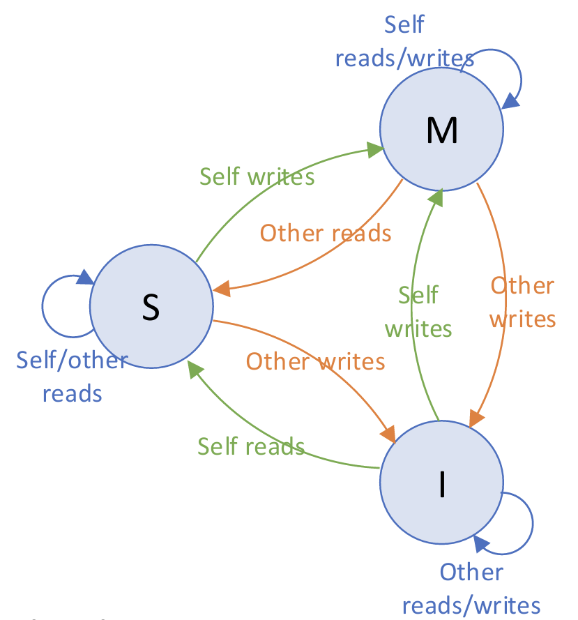
Self read/write triggers up transition, while ther read/write triggers down transition.

Downgrading from M (to S or I) causes writeback.

Implementation

In each cache entry, extend the valid bit to represent 3 states: M, S, or I

Each private cache needs to be told the actions of others, how?

• Choice 1: snooping
  • All caches broadcast their misses through the interconnect
  • Each cache “snoops” all events from all cores
• Choice 2: directory-based
  • Use a directory to track the state of each block, e.g., who are the sharers
  • The directory tells the sharers, i.e., those who have the block and need to respond, when necessary
  • Benefits: reduce messages (to only relevant sharers)

In both cases, different blocks take independent coherence actions.

False Sharing: different memory locations, mapped to same cache block. This is the artifactual effect due to the granularity of coherence tracking. Can be reduced by software techniques, e.g., padding.

On-Chip Networks

Banked Caches

Large (shared) caches are usually implemented with banking. Each bank is like an individual cache, but is smaller and placed closer to each core. Note that each cache block can only reside in only one of the banks at any time. Benefits: lower hit latency, more parallelism

Mapping policy: block address → bank index

• Static: block address decides which bank the block should be stored in. E.g., bank ID is taken from lower bits in block address
• Dynamic: a block is preferred to be placed in the bank closer to the core with the most accesses to it, and may also be migrated between banks

Banking and set-associative are similar ideas at different levels!

The idea of On-Chip Networks

With many cores and their private/shared caches, we need a network to transport data blocks and coherence messages between them

On-chip network, a.k.a., network-on-chip (NoC)

• Topology: how to connect the nodes?
• Routing: which path should a message take?
• Flowcontrol: how to control actual message transport?
• Router microarchitecture: how to build the router

Transport levels:

• Message: high-level data. Software or system level, arbitrary size
• Packet: network-level object. Variable size, but bounded
• Flit: switch-level object. Fixed size, unit of flow control
• Phit: link-level object. Fixed size, usually the same size as flits, unit of data transferred on link per cycle

Zero-load latency = header latency \(T_h\) + serialization latency \(T_s\)

• Header latency \(T_h=H\times (t_r+t_l)\), where \(H\) is the number of hops, \(t_r\) is the router delay per hop, and \(t_l\) is the link delay per hop
• Serialization latency \(T_s= \frac{L}{B}\), where \(L\) is the packet size, and \(B\) is the link bandwidth

Real latency = zero-load latency + queuing delay. The latter can largely dominate!

Topology

Common topology examples:

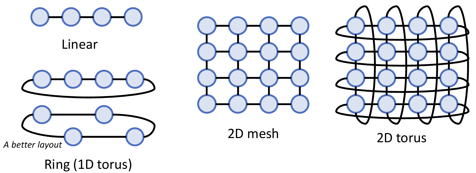
Basic definitions:

• Routing distance: number of hops on a route from source to destination
• Diameter: maximum routing distance
• A network is partitioned by a set of links if their removal disconnects the graph
• Bisection bandwidth: bandwidth crossing a minimal cut that partitions the network in two equal-sized halves

Routing

Routing chooses path that packets should follow to get from src to dst.

Properties

• Deterministic: always select the same path every time
• Minimal: only select a shortest path
• Oblivious: route is decided without considering current network state such as traffic congestion
• Deterministic routing is oblivious; oblivious routing may not be deterministic (Q: Example?)
• Adaptive (the opposite of oblivious): route is influenced by current network state, e.g., choosing a less congested route
• Source: entire route is determined at the source
• Incremental (the opposite of source): the route is incrementally determined at each hop

Dimension-Order Routing for Mesh/Torus: Resolve each dimension in a fixed order. M inimal, oblivious and deterministic (break tie for torus).

Adaptive Routing for Mesh:

• Minimal adaptive: at each hop, choose the output with the lowest load along a minimal path
• Fully adaptive: choose the output with the lowest load at each hop, take any path necessary. May encounter livelock!

Flow Control

Flow control allocates resources for packets to traverse along the route. Contention between packets causes resource conflicts, so we need flow control to manage resource allocation.

Bufferless protocols:

• Dropping: simply drop the packet if it loses resource arbitration
• Misrouting: intentionally route the losing packet away
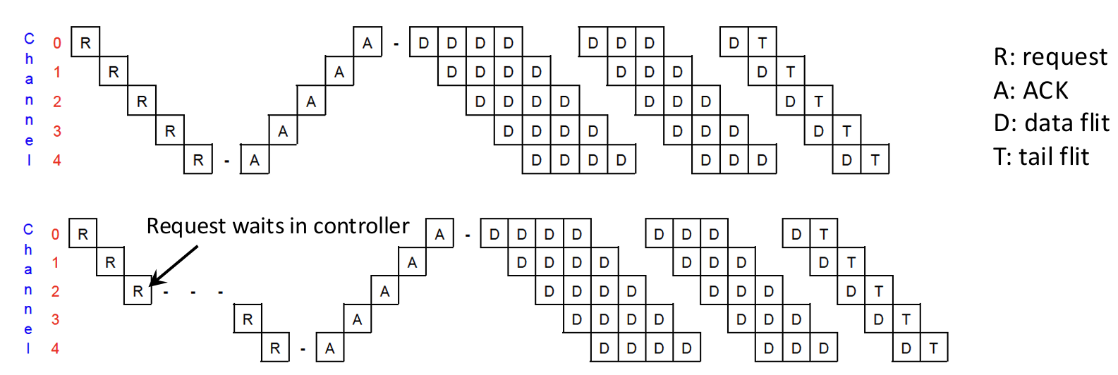
• Circuit-switching: before transmitting, use a request to set up a path and reserve all links. Then send data through the reserved path. Tail flit releases resource.

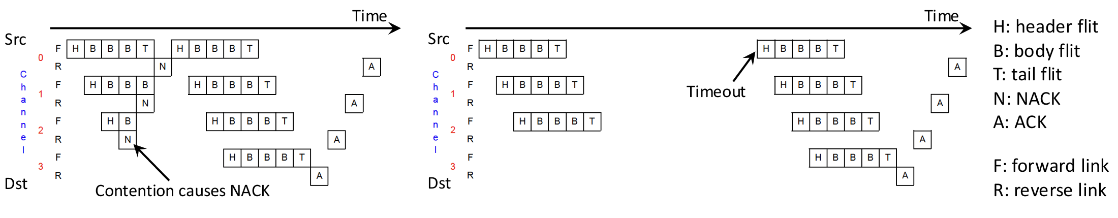
Buffered protocols allow packets to temporarily wait inside intermediate routers if encountering contention

Packet Granularity: Allocate buffer and link in unit of packets

• Store-and-forward: entire packet is stored in router before forwarding
• Cut-through: start forwarding as soon as header arrives
  Flit Granularity: Allocate buffer and link in unit of flits
• Wormhole: like cut-through, but with buffer space allocated to flits
  • head-of-line blocking when waiting in the same buffer
• virtual-channel: Provision multiple virtual channels per physical port.

If downstream has nobuffer space, backpressure informs the upstream
router to stop sending the next packet/flit. How to implement backpressure?

• Credit-based flow control: each upstream router keeps a counter of available buffer slots in downstream router. Decrement on sending, increment on receiving credit.

Deadlock and Avoidance

Resource dependency: a resource \(R_i\) is dependent on a resource \(R_j\) if it is
possible for \(R_i\) to be held by an agent \(A\) and for \(A\) to wait for \(R_j\), denoted
as \(R_i \succ R_j\).

Reason of deadlock: cyclic resource dependency. We want to avoid deadlock by eliminating all cycles.

Dimension-order routing:

• XY routing / YX routing: first resolve X / Y dimension, then Y / X dimension
• Six-turn model: At least one turn in each cycle must be disallowed to avoid cycles

Another way is resource ordering, i.e., impose a partial order on resources, and then
enforce allocating resource in non-descending order.

Example: when going from a router to the next, require VC ID to be non-descending.

Virtualization

Take physical resources (e.g., memory, processor) and transform it into a more general, flexible, and easy-to-use virtual form.

An OS supports multiple users and multiple programs on one hardware through the abstraction of processes. Schedule processes to hardware cores at different time and provide a private virtual address space to each process.

Page Table

Each process has its own virtual address space, determined by ISA. The hardware system has a single physical address space.

Page table translates virtual addresses to physical addresses, in unit of pages.

• Each process has its own page table, managed by OS, used by hardware
• Page table is stored in main memory, its base address is kept in a special register

One page table entry (PTE) per virtual page, includes: valid bit, physical page number (a.k.a., frame number), metadata (e.g., R/W/X permissions)

For a process, usually only a subset of its virtual pages are allocated, and only a subset of allocated virtual pages are mapped. Allocated but unmapped pages are swapped out to external storage, e.g., disks or SSDs.

DRAM is like a software-managed cache of disks/SSDs. Page table, managed by OS, always knows the data location

• Allocated and mapped: page hit in DRAM
• Allocated but not mapped (swapped-out): page miss, need to fetch from disk/SSD
• Unallocated: invalid access

Demand paging: if a page fault occurs, the page is paged in on demand, by the page fault handler in OS kernel.

Translation Process:

• Hardware looks up page table using virtual address
• If it is a valid page in memory
  • Check access permissions (R, W, X) against access type
  • If allowed, translate to physical address and access memory
  • Otherwise, generate a permission fault, i.e., an exception, handled by OS
• Otherwise, page is not currently in memory
  • Generate a page fault, i.e., an exception, handled by OS
  • If it is due to program errors, e.g., unallocated: terminate process
  • If page is on external storage: refill & retry, i.e., demand paging

Translation Alias:

• Synonym: a process may use different virtual addresses to point to the same physical address
• Page sharing: different processes can (read-only) share a page by setting virtual addresses to point to the same physical address
• Homonym: different processes can use the same virtual address, but actually translated to different physical addresses

Multi-Level Page Tables

Page table is sparse, only a small fraction of pages are actually allocated.

We can use a hierarchical page table structure, i.e., a (sparse) radix tree. Only top level must be resident in memory, remaining levels can be in memory or on disk, or unallocated if corresponding ranges of the virtual address space are not used.

• Advantage: save significant page table size
• Disadvantage: multiple page faults (slow)

Translation Look-aside Buffer

TLB: a hardware cache just for translation entries, i.e., PTEs.

Each TLB entry stores a page table entry (PTE) as its data,and the metadata of TLB entry itself.

If we miss in TLB, access PTE in memory. This is called page table walk.

• If page is in memory, copy PTE into TLB and retry
• If page is not in memory, raise a page fault first, then fill in TLB

When multiple processes share a processor, the OS must flush the TLB entries at context switch. Alternatively, add a process ID (PID) in each TLB entry.

The capacity of TLB is usually small. We can use multi-level TLBs, or support multiple page sizes to improve TLB reach.

Combined with Caches:

How to parallelize TLB and cache access?

Virtual Caches

Virtually indexed, virtually tagged:

• Issue 1: homonym (same virtual address, different physical addresses). Can be resolved by flushing cache on context switch or adding process ID to tags

• Issue 2: synonym (different virtual addresses, same physical address). Two copies co-exist in cache, which should be the same (physical) data. But writes to one copy will not be reflected in the other copy. This is a coherence issue in a single cache, rather than across multiple private caches, which is hard to resolve.

Instead, we choose to virtually indexed, physically tagged:

We want cache lookup index only uses bits from page offset, that is, Cache size / associativity == set size \(\le\) page size.

With this requirement, VIPT caches are functionally equivalent to PIPT caches.

Virtual Machine

How about virtualize an entire physical machine?

Virtual machine techniques honor existing hardware interface to create virtual machines.

Key requirements

• Fidelity: equivalence of interface as real physical machine
• Performance (efficiency): minimal overheads
• Safety (resource control): isolation among VMs; complete control of resources

Terminology

• Host: the underlying physical hardware system
• Guest: each VM, i.e., a virtual instance of the host
• Virtual machine monitor (VMM), a.k.a., hypervisor: the layer of software that supports virtualization

VMM Types:

• Type 0 hypervisor: hardware-based solutions; hypervisor in firmware
• Type 1 hypervisor: OS-like software; "the datacenter OS"
• Type 2 hypervisor: simply a process on host OS

Advantages:

• Easy development and testing
• Server consolidation: improve utilization
• Live migration: for elastic scale-down and load balance
• Security: strong isolation between VMs even on the same machine

VM vs. hypervisor is similar to process vs. OS. Consider: Time multiplexing, e.g., for processor cores; Resource partitioning, e.g., for physical memory, disks; Mediating hardware interface, e.g., for networking, keyboard/mouse

Compatibility Options:

• Paravirtualization
  • Whether running within a hypervisor or directly on host is transparent to apps but not guest OS, i.e., guest OS needs to be modified
  • Advantage: simpler to implement; smaller performance overheads
  • Disadvantage: cannot be used for arbitrary OS'es, e.g., close-source Windows
• Full virtualization
  • Transparent to both guest OS and apps
  • Advantage: work without any changes
  • Disadvantage: performance overheads must be paid to address issues

Privilege Mode

VMM runs in kernel mode with high privilege. Physical user mode is divided to virtual user mode and virtual kernel mode. Guest apps run in virtual user mode and guest OS run in the virtual kernel mode.

Trap-and-Emulate

• When a guest app in physical user mode wants to execute a privilege instruction, it traps into physical kernel mode, i.e., VMM.
• VMM executes (i.e., emulate) the actions on behalf of guest OS.
• VMM returns to guest OS and updates guest OS states
• Guest OS returns to guest app

Trap-and-emulate requires all sensitive instructions are privileged. However, this is not true for some architectures, e.g., x86.

• Solution 1: use paravirtualization
• Solution 2: binary translation: VMM examine severy instruction, dynamically rewrites binary to translate sensitive but not privileged instructions to emulation code
• Solution 3: hardware support: New operating modes, e.g., VT root mode for VMM and non-root mode for guest OS. New instructions to transition between modes.

Address Translation

Guest virtual address (gVA) → guest physical address (gPA) == Host virtual address (hVA) → host physical address (hPA)

Nested page tables, a.k.a., extended page tables in Intel

• Use page tables in guest OS to translate gVA → gPA
• Use page table in VMM to translate gPA → hPA

TLB entries directly cache gVA → hPA. Tagged TLB with VM IDs, so no need to flush TLB on VM transitions.

Page table walk becomes nested 2D! Support 2D page table walk in hardware.

Shadow Page Tables: map gVA → hPA directly

• VMM creates and manages
• One shadow pagetable per guest app
• used by hardware

VMM needs to keep shadow pagetable consistent with page table in guest OS

• Advantages: fast page table walk, require little hardware support
• Disadvantages: more traps for page table updates, storage overheads