[Subfield] Selfish Routing

Selfish Routing

Non-atomic Routing Model

Routing Game and Flows

You are given a directed network \(G=(V,E)\) and \(k\) source-destination vertex pairs \(\{s_1,t_1\},\ldots,\{s_k,t_k\}\), also called commodities. We denote the set of (simple) \(s_i-t_i\) paths by \(\mathcal{P}_i\), and define \(\mathcal{P} = \cup_i \mathcal{P}_i\).

A flow is a function \(f:\mathcal{P}\rightarrow\mathbb{R}^+\); for a fixed flow \(f\) we define \(f_e = \sum_{P:e\in P} f_P\). We associate a finite and positive rate \(r_i\) with each pair \(\{s_i,t_i\}\), the amount of flow with source \(s_i\) and destination \(t_i\). A flow \(f\) is said to be feasible if for all \(i\), \(\sum_{P\in\mathcal{P}_i} f_P = r_i\).

To capture the congestion, each edge \(e\in E\) is given a load-dependent latency function that we denote by \(\ell_e(\cdot)\). For each \(e\in E\), we assume that the latency function \(\ell_e\) is nonnegative, differentiable, and nondecreasing. The latency of a path \(P\) with respect to a flow \(f\) is defined as the sum of the latencies of the edges in the path, denoted by \(\ell_P(f) = \sum_{e\in P} \ell_e(f_e)\). We define the cost \(C(f)\) of a flow \(f\) in \(G\) as the total latency incurred by \(f\), that is,

\[C(f) = \sum_{P\in\mathcal{P}} \ell_P(f) f_P = \sum_{e\in E} \ell_e(f_e) f_e. \]

Optimal flows are flows that minimize the cost $C(f)$ over all feasible flows. Equivalently, optimal flows are the solutions to the following non-linear programming: $$ (NLP)\qquad\qquad\qquad\qquad\begin{align*} \min \quad & \sum_{e\in E} \ell_e(f_e) \\ \text{s.t.} \quad & \sum_{P\in\mathcal{P}_i} f_P = r_i, && \forall i\in\{1,\ldots,k\} \\ & f_e = \sum_{P\in\mathcal{P}:e\in P} f_P, && \forall e\in E \\ & f_P \geq 0, && \forall P\in\mathcal{P} \end{align*}\qquad\qquad\qquad\qquad\qquad\qquad $$

The flow $f$ is optimal for a convex program of the form (NLP) if and only if for every $i\in\{1,\ldots,k\}$ and $P_1,P_2\in\mathcal{P}_i$ with $f_{P_1}>0$, $c_{P_1}'(f) \leq c_{P_2}'(f)$.

In our problem, \(\ell_e(f_e)=\ell_e(f_e)f_e.\) Denote marginal cost function as \(\ell^*_e(f_e)=\ell_e'(f_e)=\ell_e(f_e)+\ell'_e(f_e)f_e.\)

Without central supervision, the flow will form Nash equilibrium:

A flow $f$ feasible for instance $(G,r,\ell)$ is at Nash equilibrium if and only if for every $i\in\{1,\ldots,k\}$ and $P_1,P_2\in\mathcal{P}_i$ with $f_{P_1}>0$, $\ell_{P_1}(f) \leq \ell_{P_2}(f)$. Such $f$ is also called a Nash flow.

A flow $f$ for instance $(G,r,\ell)$ is at Nash equilibrium if and only if $$ \sum_{e\in E}\ell_e(f_e)f_e\le \sum_{e\in E}\ell_e(f_e)f_e^* $$ for every feasible flow $f^*$.

An instance $(G,r,\ell)$ with continuous, nondecreasing latency functions admits a feasible flow at Nash equilibrium. Moreover, if $f$, $\tilde{f}$ are flows at Nash equilibrium, then $\ell_e(f_e)=\ell_e(\tilde{f}_e)$ for all edges $e$ and $C(f) = C(\tilde{f})$.

Let $h_e(x)=\int_0^x\ell_e(t)\mathrm{d}t$. We can see that $h_e$ is convex. Consider the convex program $$ (NLP2)\qquad\qquad\qquad\qquad\begin{align*} \min \quad & \sum_{e\in E} h_e(f_e) \\ \text{s.t.} \quad & \sum_{P\in\mathcal{P}_i} f_P = r_i, && \forall i\in\{1,\ldots,k\} \\ & f_e = \sum_{P\in\mathcal{P}:e\in P} f_P, && \forall e\in E \\ & f_P \geq 0, && \forall P\in\mathcal{P} \end{align*}\qquad\qquad\qquad\qquad\qquad\qquad $$ By Lemma, the optimal solutions for (NLP2) are precisely the flows at Nash equilibrium for $(G,r, \ell)$. Existence of a Nash equilibrium follows from the facts that (NLP2) has a continuous objective function and a compact feasible region.

Next, suppose \(f\), \(\tilde{f}\) are flows in \(G\) at Nash equilibrium (and hence global optima for (NLP2)). By convexity of the objective function of (NLP2), whenever \(f_e \neq \tilde{f}_e\) the function \(h_e\) must be linear between these two values (since any convex combination would yield a solution for (NLP2) with smaller objective function value) and hence \(\ell_e\) must be constant between these two values. This implies that \(\ell_e(f_e) = \ell_e(\tilde{f}_e)\) for all \(e \in E\), thus \(C(f) = C(\tilde{f})\).

Besides, there are some useful properties of Nash equilibrium in single-commodity networks.

Let $(G,r,\ell)$ be an single-commodity instance. There is a constant $c(G,r,\ell)\ge 0$ such that for any Nash equilibrium $f$ for $(G,r,\ell)$ and any $P\in\mathcal{P}$ with $f_P>0$, $\ell_P(f)=c(G,r,\ell)$. Furthermore, $c(G,r,\ell)$ is nondecreasing in $r$.

Let $(G,r,\ell)$ be an single-commodity instance and $f$ a feasible flow for $(G,r,\ell)$. For each vertex $v$ in $G$, let $d(v)$ denote the shortest-path distance from $s$ to $v$ with respect to edge lengths $\ell_e(f_e)$ in $G$. Then, $f$ is a Nash equilibrium if and only if for all edges $e=(v,w)$, either $f_e=0$ or $d(w)-d(v)=\ell_e(f_e).$

Every single-commodity instance admits a directed acyclic Nash equilibrium.

Price of anarchy and Pigou Bound

The price of anarchy (PoA) is a measure to quantify the efficiency loss caused by selfish behavior. In the context of network routing games, it is defined as the worst-case ratio over all instances between the cost of a Nash flow and the cost of an optimal flow. Formally,

The PoA of a class of instances $\mathcal{I}$ is defined as $$ \text{PoA}(\mathcal{I}) = \sup_{(G,r,\ell)\in\mathcal{I}} \frac{\max_{f\text{ at Nash equilibrium}} C(f)}{\min_{f\text{ feasible}} C(f)}. $$

Pigou bound measures PoA well.

Let $\mathcal{C}$ be a set of cost functions. The Pigou bound $\alpha(\mathcal{C})$ for $\mathcal{C}$ is defined as $$ \alpha(\mathcal{C})=\sup_{c\in\mathcal{C}}\sup_{x,r\ge 0}\frac{r\cdot c(r)}{x\cdot c(x)+ (r-x)c(r)} $$ with the understanding that $0/0=1$.

For example, if \(\mathcal{C}\) is the set of polynomials with nonnegative coefficients and degree at most \(p\), then

\[\alpha(\mathcal{C})=\left(1-p(p+1)^{-(p+1)/p}\right)^{-1}. \]

As \(p\to \infty\), it tends to infinity as \(p/\ln p\).

Let $\mathcal{C}$ be a set of cost functions that contains all of the constant cost functions, then:

• the PoA of instances with cost functions in \(\mathcal{C}\) is at most \(\alpha(\mathcal{C})\);
• the PoA of instances with cost functions in \(\mathcal{C}\) can be arbitrarily close to \(\alpha(\mathcal{C})\).

Let $\mathcal{C}$ be a set of functions that contains all of the constant functions and $\alpha(\mathcal{C})$ the Pigou bound for $\mathcal{C}$. By definition, for $c\in \mathcal{C}$ and $x,r\ge 0$, $$ x\cdot c(x)\ge \frac{r\cdot c(r)}{\alpha(\mathcal{C})}+(x-r)c(r) $$ Let $f$ and $f^*$ be an optimal flow and a Nash equilibrium, respectively, for an instance $(G,r,c)$ with cost functions in $\mathcal{C}$. We have $$ \begin{align*} C(f^*)= &\ \sum_{e\in E}\ell_e(f_e^*)f_e^*\\ \ge &\ \frac{1}{\alpha(\mathcal{C})}\sum_{e\in E}\ell_e(f_e)f_e+\sum_{e\in E}(f_e^*-f_e)\ell_e(f_e)\\ \ge &\ \frac{C(f)}{\alpha(\mathcal{C})}. \end{align*} $$ On the other hand, the following construction can be infinitely close to the Pigou bound, where the optimal solution is $\inf\limits_{x,r\ge 0} \left(x\cdot c(x)+(r-x)c(r)\right)$ and the Nash equilibrium is $r\cdot c(r)$.

PoA can be super large when cost functions are highly non-linear! How can we reduce it?

Edge Removal

The Brays paradox shows that removing edges from a network may improve its performance. This fact leads to consideration of the problem called NETWORK DESIGN: given a network, which edges should be removed to obtain the best flow in Nash equilibrium? Similarly, given a large network of candidate edges to be built, which subnetwork will show the best performance when used selfishly?

We study how much this mechanism can improve the efficiency of Nash equilibrium.

Single-commodity Networks

The Braess ratio $\beta(G,r,\ell)$ of a single-commdity instance $(G,r,\ell)$ is $$ \beta(G,r,\ell)=\max_{H\subseteq G}\frac{C(f)}{C(f^H)}, $$ where $f$ and $f^H$ denote Nash equilibria for $(G,r,\ell)$ and $(H,r,\ell)$, respectively.

Clearly, \(\beta(G,r,\ell)\le \text{PoA}(G,r,\ell)\).

First, we can construct a family of instances with arbitrarily large Braess ratio.

For every $n\ge 2$, there is a single-commodity instance $(G,r,\ell)$ with $n$ vertices and $$\beta(G,r,\ell)\ge\left\lfloor\frac{n}{2}\right\rfloor.$$

Only need to consider the case $n=2k+2$ for positive integer $k$. Let's define the $k$-th Braess graph $B^k=(V^k,E^k)$:

• \(V^k=\{s, v_1,...,v_k,w_1,...,w_k,t\}\)
• \(E^k=\{(s,v_i),(v_i,w_i),(w_i,t): 1\le i\le k\}\cup \{(v_i,w_{i-1}):2\le i\le k\}\cup\{(v_1,t),(s,w_k)\}\)

Call edges of form \((v_i,w_i)\) the type A edges, edges of form \((v_i,w_{i-1}),(v_1,t),(s,w_k)\) the type B edges, and edges of form \((s,v_i)\), \((w_i,t)\) the type C edges. Let their latency functions be defined as follows:

• Type A edges: \(\ell_e^k(x)=0\);
• Type B edges: \(\ell_e^k(x)=1\);
• Type C edges: For each \(i\in\{1,2,...,k\}\), \(e\in \{(w_i,t),(s,v_{k-i+1})\}\), \(\ell^k_e(x)\) is an arbitrary continuous, nondecreasing latency function that \(\ell_e^k(x)=0\) for \(x\le k/(k+1)\) and \(\ell_e^k(x)=i\) for \(x\ge 1\).

For \(i=1,...,k\), let \(P_i\) denote the path \(s\to v_i\to w_i\to t\). For \(i=2,...,k\), let \(Q_i\) denote the path \(s\to v_i\to w_{i-1}\to t\). Define \(Q_1\) to be the path \(s\to v_1\to t\) and \(Q_{k+1}\) the path \(s\to w_k\to t\). Routing one unit flow on each of \(P_1,...,P_k\) yields a Nash equilibrium for \((B^k,k,\ell^k)\) and routing one \(\frac{k}{k+1}\) unit of flow on each of \(Q_1,...,Q_{k+1}\) yields a Nash equilibrium for \((H,k,\ell^k)\) where \(H\) is the subgraph obtained from \(B^k\) by deleting the \(k\) type A edges. One can verify that the total latency of these two flows are \(k(k+1)\) and \(k\), respectively. Thus

\[\text{PoA}(B^k,k,\ell^k)=k+1=n/2. \]

Next, let's see an upper bound for Braess ratio. It shows that Braess ratio is maximized by the instances constructed in the previous theorem.

Let's begin with defining some combinatorial structure.

Let $f$ and $\tilde{f}$ be feasible flows for the instance $(G,r,c)$.

• An edge \(e\) of \(G\) is
  • \((f,\tilde{f})\)-light if \(f_{e} \leq \tilde{f}_{e}\) and \(\tilde{f}_{e} > 0\),
  • \((f,\tilde{f})\)-heavy if \(f_{e} > \tilde{f}_{e}\),
  • \((f,\tilde{f})\)-useless if \(f_{e} = \tilde{f}_{e} = 0\).
• An undirected path is \((f,\tilde{f})\)-alternating if it comprises only:
  • forward \((f,\tilde{f})\)-light edges and
  • backward \((f,\tilde{f})\)-heavy edges.

Let $f$ and $\tilde{f}$ be flows feasible for the single-commodity instance $(G, r,\ell)$. Then, there is an $(f, \tilde{f})$-alternating $s$-$t$ path. Moreover, if $f$ is directed acyclic, then every such path begins and ends with an $(f, \tilde{f})$-light edge.

Assume that there is no $(f, \tilde{f})$-alternating $s$-$t$ path and let $S$ denote the set of nodes reachable from $s$ via such paths. Then $S$ is an $s$-$t$ cut, the flow that $f$ and $\tilde{f}$ exiting $S$ is exactly $r$.

Since vertices in \(S\) can be reached from \(s\) via \((f, \tilde{f})\)-alternating paths and vertices outside \(S\) cannot, edges that exit \(S\) cannot be \((f, \tilde{f})\)-light, and edges that enter \(S\) cannot be \((f, \tilde{f})\)-heavy. Since the flow across \(S\) is positive (assuming \(r > 0\)), some non-useless (and thus heavy) edge exits \(S\). Taken together, these facts imply that \(f\) exiting \(S\) is strictly greater than \(\tilde{f}\) exiting \(S\), which leads to contradiction.

Moreover, if \(f\) is directed acyclic, then it sends no flow into \(s\) or out of \(t\). Thus, the first and last edges of every \((f, \tilde{f})\)-alternating \(s\)-\(t\) path must be \((f, \tilde{f})\)-light.

Let $(G,r,\ell)$ be a single-commodity instance and $S$ a subset of the edges of $G$. The set $S$ is sparse if no two edges of $S$ share an endpoint, and in addition no edge of $S$ is incident to $s$ or $t$.

In other words, a sparse edge set is a matching of $V\setminus\{s,t\}$.

The following theorem provides a general upper bound for Braess ratio with respect to the size of sparse edge sets in the network.

Let $(G, r,\ell)$ be a single-commodity instance, $H$ a subgraph of $G$, and $f$ and $f^H$ Wardrop equilibria for $(G, r,\ell)$ and $(H, r,\ell)$, respectively. Let $S$ denote the edges in $G$ but not $H$. If every sparse subset of $S$ contains at most $k$ edges, then $$ C(f) \leq (k + 1) \cdot C(f^H). $$

Let $f$ be a directed acyclic Wardrop equilibrium for $(G, r,\ell)$ and $\tilde{f}$ a Nash equilibrium for $(H, r,\ell)$. For each vertex $v$, let $d(v)$ denote the shortest-path distance from $s$ to $v$ with respect to edge lengths $\ell_e(f_e)$ in $G$, and $\tilde{d}(v)$ the $s$-$v$ distance with respect to $\ell_e(\tilde{f}_e)$ in $H$. By definition of Nash equilibrium, $f$ and $\tilde{f}$ only have flows on the corresponding shortest paths. Obviously, $C(f) = r \cdot d(t)$ and $C(\tilde{f}) = r \cdot \tilde{d}(t)$, so the theorem reduces to proving that $d(t) \leq (k + 1) \cdot \tilde{d}(t)$, where $k$ is the size of some sparse set of edges present in $G$ but not $H$.

By lemma, there exists an \((f, \tilde{f})\)-alternating \(s\)-\(t\) path, denoted by \(P\). A segment of \(P\) is a maximal subpath of \(P\) that contains only \((f, \tilde{f})\)-light or only \((f, \tilde{f})\)-heavy edges. Edges that are in \(G\) but not \(H\) are called absent, can only reside in \((f, \tilde{f})\)-heavy segments. The key claim is that if \(v\) is a vertex at the end of a segment of \(P\), and \(i\) (heavy) segments of \(P\) between \(s\) and \(v\) contain an absent edge, then

\[d(v) \leq \tilde{d}(v) + i \cdot \tilde{d}(t).\tag{claim} \]

Let's prove it by induction on the segments of \(P\). The inequality trivially holds when \(v = s\), so suppose it holds for a vertex \(v\) that is last on a segment of \(P\), or is the source \(s\). We wish to prove (claim) for \(w\), defined as the last vertex on the next segment. Let \(i\) denote the number of earlier segments of \(P\) that contain at least one absent edge. By the inductive hypothesis, \(d(v) \leq \tilde{d}(v) + i \cdot \tilde{d}(t)\). The inductive step has two cases:

• For the first case, suppose that the segment between \(v\) and \(w\) contains at least one absent edge. As absent edges can only be \((f, \tilde{f})\)-heavy, this segment comprises only \((f, \tilde{f})\)-heavy backward edges. We can see that

\[d(w) \leq d(v) \leq \tilde{d}(v) + i \cdot \tilde{d}(t) \leq (i + 1) \cdot \tilde{d}(t) \leq \tilde{d}(w) + (i + 1) \cdot \tilde{d}(t). \]

• For the second case of the inductive step, suppose that the current segment \(Q \subseteq P\) contains no absent edges. We will prove, by induction on the vertices of \(Q\), that

\[d(x) \leq \tilde{d}(x) + i \cdot \tilde{d}(t) \]

for all vertices \(x\) of \(Q\). Suppose \(d(x) \leq \tilde{d}(x) + i \cdot \tilde{d}(t)\) for a vertex \(x\) of \(Q\) and let \(y\) denote the next vertex on the segment.

• If the edge \((x, y) \in P\) is \((f, \tilde{f})\)-light, then \(\ell_e(f_e) \leq \ell_e(\tilde{f}_e)\) and \(f_e > 0\). Since \(f\) and \(\tilde{f}\) are Wardrop equilibria, we have

\[d(y) = d(x) + \ell_e(f_e) \leq \tilde{d}(x) + \ell_e(\tilde{f}_e) + i \cdot \tilde{d}(t) = \tilde{d}(y) + i \cdot \tilde{d}(t). \]

• If the edge \(e = (y, x) \in P\) is \((f, \tilde{f})\)-heavy, then

\[d(y) = d(x) - \ell_e(f_e) \leq \tilde{d}(x) + i \cdot \tilde{d}(t) - \ell_e(\tilde{f}_e) \leq \tilde{d}(y) + i \cdot \tilde{d}(t). \]

In either case, the inductive step holds.

Finally, let's see how this claim implies the theorem. Directly apply it to \(t\) to obtain

\[d(t) \leq \tilde{d}(t) + k \cdot \tilde{d}(t) = (k + 1) \cdot \tilde{d}(t), \]

where \(k\) is the number of segments of \(P\) that include an absent edge. Again by lemma, the \((f,\tilde{f})\)-heavy segments of \(P\) are disjoint from each other and from \(s\) and \(t\). Picking one absent edge from each of these \(k\) segments that include an absent edge, we obtain a sparse set of edges in \(G\) that contains at most \(k\) edges. Thus, the theorem holds.

Let $(G, r,\ell)$ be a single-commodity instance with $n$ vertices, then $$ \beta(G,r,\ell)\le \left\lfloor\frac{n}{2}\right\rfloor. $$

Multi-commodity Networks

For multi-commodity networks, the Braess ratio is defined as follows:

The Braess ratio $\beta(G,r,\ell)$ of a multi-commodity instance $(G,r,\ell)$ is $$\beta(G,r,\ell)=\max_{H\subseteq G}\min_{i=1}^k\frac{C_i(f)}{C_i(f^H)},$$ where $f$ and $f^H$ denote Nash equilibria for $(G,r,\ell)$ and $(H,r,\ell)$, respectively, and $C_i(f)$ is the cost of commodity $i$ with respect to flow $f$.

The lower bound is exponential in the network size, even for two-commodity networks.

There is a family of two-commodity instances $\{(G^n,r^n,\ell^n)\}_{n\ge 1}$ such that the size of $G^n$ is $O(n)$, and $\beta(G^n,r^n,\ell^n)=2^{\Omega(n)}$ as $n\to \infty$.

On the other hand, it's at most exponential in the network size.

There is a constant $c>0$ such that for every $k,n\ge 1$ and every instance $(G,r,\ell)$ with $k$ commodities and $n$ vertices, $\beta(G,r,\ell)\le 2^{ckn}$.

Detecting Braess Paradox Is Hard

So far, we have studied the possible benefits of Edge Removal. But how do we get this benefit? From an algorithmic perspective, we want to efficiently find the edges to remove so that the Nash equilibrium has the minimum cost. Here we only consider the single-commodity case. We will show the hardness of this problem.

LINEAR NETWORK DESIGN is the problem as follows: given a single-commodity instance \((G,r,\ell)\) with linear cost functions, find a subgraph \(H\) of \(G\) such that the cost of Nash equilibrium for \((H,r,\ell)\) is minimized.

The trivial algorithm that return the entire graph is a $\frac{4}{3}$-approximation algorithm for LINEAR NETWORK DESIGN.

In fact, it's almost optimal.

For every $\epsilon>0$, there is no $\left(\frac{4}{3}-\epsilon\right)$-approximation algorithm for LINEAR NETWORK DESIGN unless $\mathsf{P=NP}$.

Let's reduce it to 2 DIRECTED DISJOINT PATHS (2DDP), which is proven to be NP-hard: given a directed graph $G$ and two pairs of vertices $(s_1,t_1)$ and $(s_2,t_2)$, decide whether there are two vertex-disjoint paths from $s_1$ to $t_1$ and from $s_2$ to $t_2$.

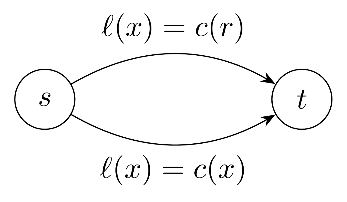
Consider an instance \(\mathcal{I}=(G,s_1,s_2,t_1,t_2)\) of 2DDP. Augment the vertex set by an additional source \(s\) and \(t\), and include the directed edges \((s,s_1),(s,s_2),(t_1,t)\) and \((t_2,t)\), with latency functions \(\ell(x)=1,\ell(x)=x,\ell(x)=1,\ell(x)=x\), respectively. And all edges in \(E\) have a latency function \(\ell(x)=0\). So far, we construct an instance \((G',1,\ell)\) for LINEAR NETWORK DESIGN in polynomial time.

We want to show that

• if \(\mathcal{I}\) is a "YES" instance, then there is a subgraph \(H\) of \(G'\) such that the cost of Nash equilibrium for \((H,1,\ell)\) is at most \(\frac{3}{2}\);
• if \(\mathcal{I}\) is a "NO" instance, then for every subgraph \(H\) of \(G'\), the cost of Nash equilibrium for \((H,1,\ell)\) is at least \(2\).

For the first statement, suppose there are vertex-disjoint \(s_1\)-\(t_1\) and \(s_2\)-\(t_2\) paths \(P_1\) and \(P_2\) in \(G\), respectively. Let \(H\) be the subgraph of \(G'\) that contains all edges of \(P_1\) and \(P_2\). Clearly, routing \(\frac{1}{2}\) flow along each path yields a Nash equilibrium with cost \(\frac{3}{2}\).

For the second statement, suppose there is no vertex-disjoint paths. Suppose \(H\) is a subgraph of \(G'\) that has an \(s\)-\(t\) path. Notice that all \(s\)-\(t\) paths \(P\) in \(H\) contain an \(s_i\)-\(t_j\) path for some \(i,j\in\{1,2\}\), routing all of the flow on \(P\) yields a Nash equilibrium with cost at least \(2\).

We have similar results for GENERAL NETWORK DESIGN, which is the version of LINEAR NETWORK DESIGN with general cost functions.

The trivial algorithm that return the entire graph is a $\left\lfloor\frac{n}{2}\right\rfloor$-approximation algorithm for GENERAL NETWORK DESIGN.

For every $\epsilon>0$, there is no $\left(\left\lfloor\frac{n}{2}\right\rfloor-\epsilon\right)$-approximation algorithm for GENERAL NETWORK DESIGN unless $\mathsf{P=NP}$.

Taxes

Another approach is to use taxes. Formally, each edge \(e\in E\) is assigned a tax \(\tau_e\ge 0\), and the latency function of edge \(e\) becomes \(\ell_e(f_e)+\tau_e\). The new instance is denoted by \((G,r,\ell+\tau)\), where \(\tau=(\tau_e)_{e\in E}\). The cost of a flow \(f\) in this new instance is defined as $$C(f,\ell+\tau) = \sum_{P\in\mathcal{P}} \ell_P(f) f_P + \sum_{e\in E} \tau_e f_e = C(f,\ell) + \sum_{e\in E} \tau_e f_e.$$ It is a generalization of edge removal, since assigning an infinite tax to an edge is equivalent to removing it.

Marginal Cost Taxes

Intuitively, marginal cost taxes \(\tau_e^m:=f_e\ell_e'(f_e)\) (where \(f\) is an optimal flow) may help since it induce the optimal flow as a Nash equilibrium.

Let $(G,r,\ell)$ be an instance and $f^*$ be an optimal flow for $(G,r,\ell)$. Let $\tau^m$ be the marginal cost tax for $(G,r,\ell)$, then $f^*$ is at Nash equilibruim for $(G,r,\ell+\tau^m)$.

However, it does not always work, for example in the case of linear latency functions.

Let $(G,r,\ell)$ be an instance with linear latency functions and $\tau^m$ be the corresponding marginal cost taxes. Let $f$ and $f^\tau$ be Nash equilibria of $(G,r,\ell)$ and $(G,r,\ell+\tau^m)$, respectively. Then, $$C(f,\ell)\le C(f^\tau,\ell+\tau^m).$$

Let $f$ and $f^*$ be a Nash equilibrium and an optimal flow for $(G,r,\ell)$, respectively. Write $\ell_e(x)=a_ex+b_e$ for each edge $e\in E$, then $\tau^m_e=a_ef^*_e$. Define $\ell^*_e$ by $\ell^*_e(x)=2a_ex+b_e$. Notice that $f/2$ is a Nash equilibrium for $(G,r,\ell^*)$, and $c(G,r,\ell)=c(G,r/2,\ell^*)$. Then we have $$c(G,r,\ell)=c(G,r/2,\ell^*)\le c(G,r,\ell^*)=c(G,r,\ell+\tau^m).$$

v.s. Edge Removal

One may ask whether arbitrary tax is really more powerful than edge removal. For the case of linear latency functions, the answer is no.

An instance with linear latency functions admits a tax $\tau$ that is $0/\infty$. We say a tax $\tau$ for instance $(G,r,\ell)$ is $0/\infty$ if, for any Nash equilibrium $f$ for $(G,r,\ell+\tau)$, $\tau_e=0$ or $f_e^\tau=0$ for each edge $e\in E$.

Assume the theorem is false. Consider the counterexample instance $(G,r,\ell)$ having as few edges as possible, admitting tax $\tau$ and Nash equilibrium $f^\tau$ for $(G,r,\ell+\tau)$ that $C(f^\tau,\tau)$ smaller than the cost of any Nash equilibrium with $0/\infty$ tax.

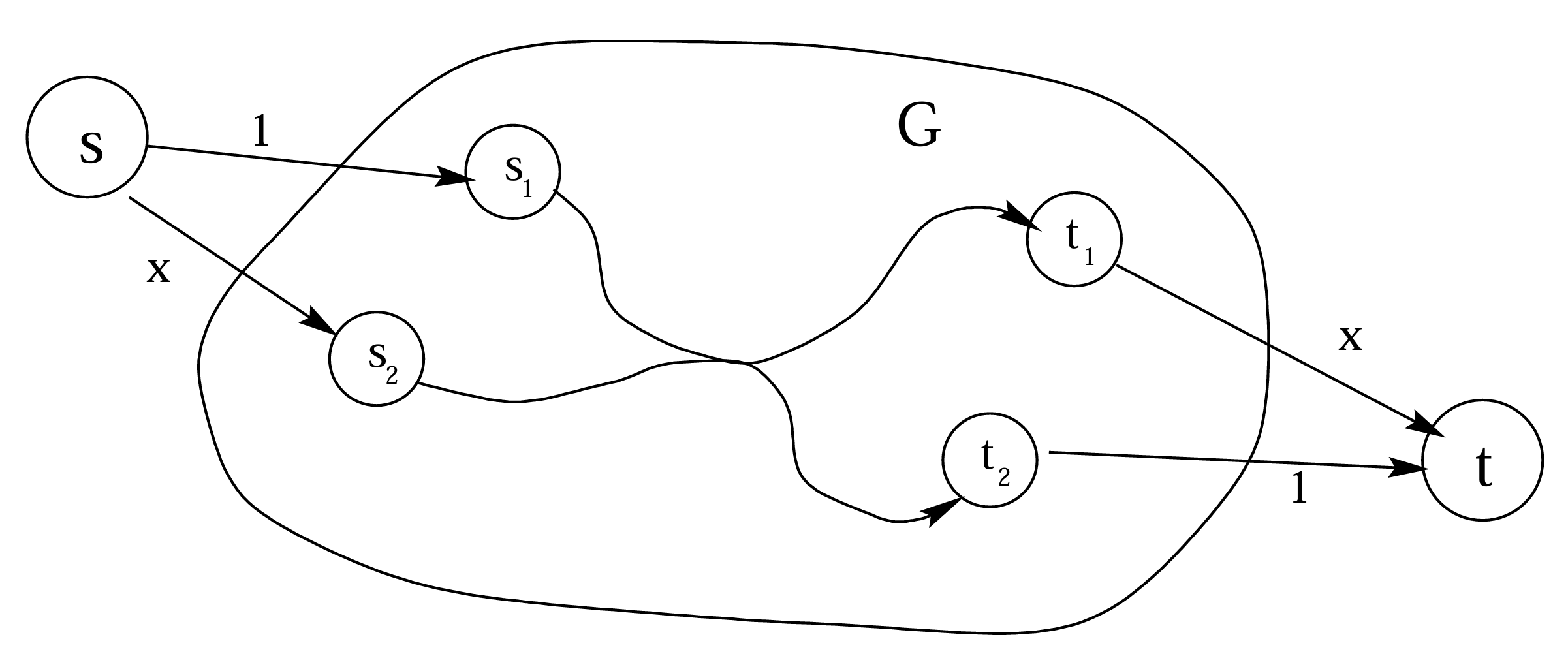
This minimal counterexample has some properties. We can see that \(f_e^\tau>0\) for all edges \(e\in E\) since otherwise we can remove the edge \(e\) with \(f_e^\tau=0\) and obtain a smaller counterexample. Combined with the proposition, \(G\) is directed acyclic. Furthermore,

The Nash equilibrium is unique. In other words, $f$ is a Nash equilibrium for $(G,r,\ell+\tau)$ if and only if $f_e=f_e^\tau$ for all edges $e\in E$.

To see this, we first apply the previous uniqueness theorem. Suppose $f$ is another Nash equilibrium, $f$ and $f^\tau$ differ only on edges with a constant latency function. It implies that $f-f^\tau$ is a circular flow. Then $f^\lambda=f^\tau+\lambda(f-f^\tau)$ is a Nash equilibrium for $(G,r,\ell+\tau)$ for sufficiently small $\lambda>0$. On the other hand, since $G$ is directed acyclic, $f_e-f^\tau_e<0$ for some edge $e\in E$. Thus we can choose $\lambda$ such that $f^\lambda$ is a Nash equilibrium but $f^\lambda_e=0$ for some edge $e\in E$, leads to contradiction.

Now return to the proof of the theorem. Write $\ell_e(x)=a_ex+b_e$ for each edge $e\in E$. The equations $$\sum_{e\in P} (a_ef_e+b_e+\tau_e)=c$$ for all $P\in\mathcal{P}$, together with the standard flow conservation constraints, form a linear system with $m+1$ variables $\{f_e\}$ and $c$ (where $m$ is the number of edges in $G$). By Lemma, it has the unique solution $(f^\tau,c^\tau)$. Choosing $m+1$ linearly independent constraints with at least one constraint corresponding to a path with nonzero tax, there is a square linear system $$A\begin{bmatrix}\ f\ \\\ c\ \end{bmatrix}=d$$ for which $\begin{bmatrix}\ f^\tau\ \\\ c^\tau\ \end{bmatrix}=A^{-1}d.$ Let $$M=\inf_{\tau \text{ is optimal for }(G,r,\ell)}\left(\sum_{e\in E}\tau_e\right).$$ Clearly, $M>0$. We can choose $\tau$ as the optimal tax for $(G,r,\ell)$ such that $\sum_{e\in E}\tau_e\le \left(1+\frac{1}{2m}\right)M$. Notice that $\tau_{\tilde{e}}\ge\frac{M}{m}$ for some edge $\tilde{e}$. Consider perturbing $\tau$ by subtracting or adding $\frac{M}{m}$ to the tax on $\tilde{e}$. These two perturbations will give two results for the right-hand side value, $d^{-}$ and $d^{+}$, respectively. Obviously, $d^{-}+d^{+}=2d.$ Let $\begin{bmatrix}\ f^-\ \\\ c^-\ \end{bmatrix}=A^{-1}d^-$ and $\begin{bmatrix}\ f^+\ \\\ c^+\ \end{bmatrix}=A^{-1}d^+$. Immediately, we have $c^-+c^+=2c^\tau$. Since $\tau$ is optimal, $c^-=c^+=c^\tau$. Now we obtain another optimal tax $\tau^-$ with $$\sum_{e\in E} \tau_e< M,$$ which leads to contradiction.

However, this fails in general.

For each integer $n\ge 2$, there is an $n$-node instance $(G,r,\ell)$ with $c(H,r,\ell)=\left\lfloor\frac{n}{2}\right\rfloor$ for all subgraphs $H$ of $G$ but $c(G,r,\ell+\tau)=1$ for some tax $\tau$.

We will make use of the Braess graph $B_k$ with new latency functions as follows:

• Type A edges: \(\ell_e(x)=0\);
• Type B edges: \(\ell_e(x)=1\) for \(x\le \frac{1}{k+1}\) and \(\ell_e(x)=\frac{n}{2}\) for \(x\ge \frac{1}{k+1}+\epsilon\);
• Type C edges: For each \(e\in \{(w_i,t),(s,v_{k-i+1})\}\), \(\ell_e(x)=0\) for \(x\le 1+\frac{1}{k+1}\), \(\ell_e(1+\frac{1}{k})=i\), and \(\ell_e(x)=\frac{n}{2}\) for \(x\ge 1+\frac{1}{k}+\epsilon\)

where \(\epsilon>0\) is a sufficiently small constant.

If we put a tax \(\tau\) of \(1\) on each type A edge and \(0\) otherwise, then the following flow is a Nash equilibrium for \((B^k,k+1, \ell+\tau)\): \(1\) unit flow on each of \(P_1,...,P_k\) and \(\frac{1}{k+1}\) units of flow on each of \(Q_1,...,Q_{k+1}\). This Nash equilibrium proves that \(c(B^k,k+1,\ell+\tau)=1\).

On the other hand, we must show that \(c(H,k+1,\ell)\ge\frac{n}{2}\) for every subgraph \(H\) of \(B^k\). If \(H\) is all of \(B^k\), then routing \(1+\frac{1}{k}\) units on each of \(P_1,...,P_k\) yields a Nash equilibrium so that \(c(H,k+1,\ell)=\frac{n}{2}\). This is still true if \(H\) only removes some type B edges.

If a type B edge carries at least \(\frac{1}{k+1}+\epsilon\) units of flow or a type C edge carries at least \(1+\frac{1}{k}+\epsilon\) units of flow, we will say that the edge is oversaturated. We will show that if \(H\) removes some type A or type C edges, then the corresponding Nash equilibrium must oversaturate some edges, which immediately implies that \(c(H,k+1,\ell)\ge\frac{n}{2}\).

Suppose \(H\) removes some type C edges. Without loss of generality, assume \((s,v_i)\) is not in \(H\). Without oversaturation, \(s\) can only send out at most \((\frac{1}{k+1}+\epsilon)+(1+\frac{1}{k}+\epsilon)(k-1)\le k(1+\epsilon)\) units of flow, which is less than the required total flow of \(k+1\).

Finally, suppose \(H\) removes some type A edges, say \((v_i,w_i)\). The vertex \(v_i\) then has at most one outgoint edge in \(H\), which must be a type B edge. If it's not oversaturated, then \((s,v_i)\) carries at most \(\frac{1}{k+1}+\epsilon\) units of flow. By a similar argument as before, some edge incident to \(s\) is oversaturated. In either case, \(c(H,k+1,\ell)\ge \frac{n}{2}\) and the proof is complete.

Hardness of Computing Optimal Tax

Regarding the hardness of computing, we have the following result:

Unless $\mathsf{P=NP}$, for any $\epsilon>0$ there is no

• \((\frac{4}{3} - \epsilon)\)-approximation algorithm for the problem of computing the optimal tax in networks with affine latency functions;
• \(o(p/\log p)\)-approximation algorithm for the problem of computing the optimal tax in networks with latency functions that are polynomials with degree \(p\) and nonnegative coefficients;
• \(O(n^{1-\epsilon})\)-approximation algorithm for the problem of computing the optimal tax in \(n\)-node networks with arbitrary latency functions.

Stackelberg Routing

Risk Model

Reference

Correa, J. R., Schulz, A. S., & Stier-Moses, N. E. (2004). Selfish routing in capacitated networks. Mathematics of Operations Research, 29(4), 961-976.

Roughgarden, T. (2002, May). The price of anarchy is independent of the network topology. In Proceedings of the thiry-fourth annual ACM symposium on Theory of computing (pp. 428-437).

Roughgarden, T. (2001, October). Designing networks for selfish users is hard. In Proceedings 42nd IEEE Symposium on Foundations of Computer Science (pp. 472-481). IEEE.

Lin, H., Roughgarden, T., Tardos, E., & Walkover, A. (2005). Braess’s paradox, Fibonacci numbers, and exponential inapproximability. In Automata, Languages and Programming: 32nd International Colloquium, ICALP 2005, Lisbon, Portugal, July 11-15, 2005. Proceedings 32 (pp. 497-512). Springer Berlin Heidelberg.

Cole, R., Dodis, Y., & Roughgarden, T. (2003, June). How much can taxes help selfish routing?. In Proceedings of the 4th ACM Conference on Electronic Commerce (pp. 98-107).

Roughgarden, T. (2005). Selfish routing and the price of anarchy. MIT press.