


SIFT原理及源码解析
本文转自:https://blog.csdn.net/xiaowei_cqu/article/details/8087239
DoG尺度空间构造
尺度空间理论
自然界中的物体随着观测尺度不同有不同的表现形态。例如我们形容建筑物用“米”,观测分子、原子等用“纳米”。更形象的例子比如Google地图,滑动鼠标轮可以改变观测地图的尺度,看到的地图绘制也不同;还有电影中的拉伸镜头等等……
尺度空间中各尺度图像的模糊程度逐渐变大,能够模拟人在距离目标由近到远时目标在视网膜上的形成过程。
尺度越大图像越模糊。
为什么要讨论尺度空间?
用机器视觉系统分析未知场景时,计算机并不预先知道图像中物体的尺度。我们需要同时考虑图像在多尺度下的描述,获知感兴趣物体的最佳尺度。另外如果不同的尺度下都有同样的关键点,那么在不同的尺度的输入图像下就都可以检测出来关键点匹配,也就是尺度不变性。
图像的尺度空间表达就是图像在所有尺度下的描述。
尺度空间表达与金字塔多分辨率表达
高斯模糊
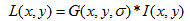
高斯核是唯一可以产生多尺度空间的核(《Scale-space theory: A basic tool for analysing structures at different scales》)。一个图像的尺度空间L(x,y,σ) ,定义为原始图像I(x,y)与一个可变尺度的2维高斯函数G(x,y,σ)卷积运算。
二维空间高斯函数:
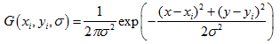
尺度空间:
尺度是自然客观存在的,不是主观创造的。高斯卷积只是表现尺度空间的一种形式。
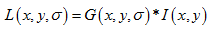
二维空间高斯函数是等高线从中心成正太分布的同心圆:
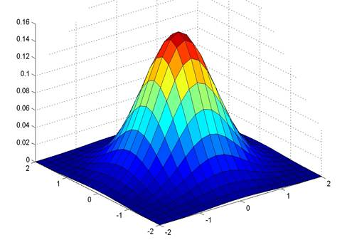
分布不为零的点组成卷积阵与原始图像做变换,即每个像素值是周围相邻像素值的高斯平均。一个5*5的高斯模版如下所示:
高斯模版是圆对称的,且卷积的结果使原始像素值有最大的权重,距离中心越远的相邻像素值权重也越小。
在实际应用中,在计算高斯函数的离散近似时,在大概3σ距离之外的像素都可以看作不起作用,这些像素的计算也就可以忽略。所以,通常程序只计算(6σ+1)*(6σ+1)就可以保证相关像素影响。
高斯模糊另一个很厉害的性质就是线性可分:使用二维矩阵变换的高斯模糊可以通过在水平和竖直方向各进行一维高斯矩阵变换相加得到。
O(N^2*m*n)次乘法就缩减成了O(N*m*n)+O(N*m*n)次乘法。(N为高斯核大小,m,n为二维图像高和宽)
其实高斯这一部分只需要简单了解就可以了,在OpenCV也只需要一句代码:
GaussianBlur(dbl, dbl, Size(), sig_diff, sig_diff);
我这里详写了一下是因为这块儿对分析算法效率比较有用,而且高斯模糊的算法真的很漂亮~
金字塔多分辨率
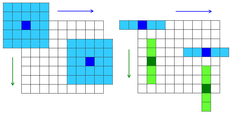
金字塔是早期图像多尺度的表示形式。图像金字塔化一般包括两个步骤:使用低通滤波器平滑图像;对平滑图像进行降采样(通常是水平,竖直方向1/2),从而得到一系列尺寸缩小的图像。
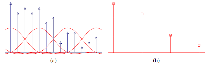
上图中(a)是对原始信号进行低通滤波,(b)是降采样得到的信号。
而对于二维图像,一个传统的金字塔中,每一层图像由上一层分辨率的长、宽各一半,也就是四分之一的像素组成:
多尺度和多分辨率
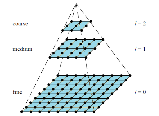
尺度空间表达和金字塔多分辨率表达之间最大的不同是:
- 尺度空间表达是由不同高斯核平滑卷积得到,在所有尺度上有相同的分辨率;
- 而金字塔多分辨率表达每层分辨率减少固定比率。
所以,金字塔多分辨率生成较快,且占用存储空间少;而多尺度表达随着尺度参数的增加冗余信息也变多。
多尺度表达的优点在于图像的局部特征可以用简单的形式在不同尺度上描述;而金字塔表达没有理论基础,难以分析图像局部特征。
DoG(Difference of Gaussian)
高斯拉普拉斯LoG金字塔
结合尺度空间表达和金字塔多分辨率表达,就是在使用尺度空间时使用金字塔表示,也就是计算机视觉中最有名的拉普拉斯金子塔(《The Laplacian pyramid as a compact image code》)。
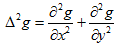
高斯拉普拉斯LoG(Laplace of Guassian)算子就是对高斯函数进行拉普拉斯变换:
核心思想还是高斯,这个不多叙述。
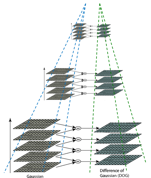
高斯差分DoG金字塔
DoG(Difference of Gaussian)其实是对高斯拉普拉斯LoG的近似,也就是对 的近似。SIFT算法建议,在某一尺度上的特征检测可以通过对两个相邻高斯尺度空间的图像相减,得到DoG的响应值图像D(x,y,σ)。然后仿照LoG方法,通过对响应值图像D(x,y,σ)进行局部最大值搜索,在空间位置和尺度空间定位局部特征点。其中:
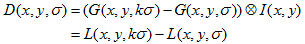
k为相邻两个尺度空间倍数的常数。
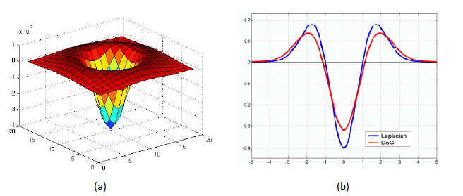
上图中(a)是DoG的三维图,(b)是DoG与LoG的对比。
金字塔构建
构建高斯金字塔
为了得到DoG图像,先要构造高斯金字塔。我们回过头来继续说高斯金字塔~
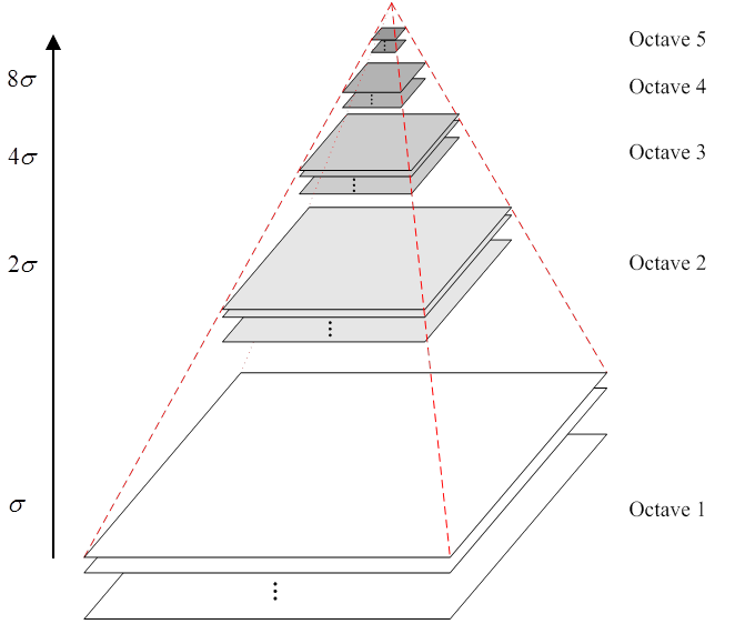
高斯金字塔在多分辨率金字塔简单降采样基础上加了高斯滤波,也就是对金字塔每层图像用不同参数的σ做高斯模糊,使得每层金字塔有多张高斯模糊图像。金字塔每层多张图像合称为一组(Octave),每组有多张(也叫层Interval)图像。另外,降采样时,金字塔上边一组图像的第一张图像(最底层的一张)是由前一组(金字塔下面一组)图像的倒数第三张隔点采样得到。
 1 void SIFT::buildGaussianPyramid( const Mat& base, vector<Mat>& pyr, int nOctaves ) const
 2 {
 3 //向量数组sig 表示每组中计算各层图像所需的方差,nOctaveLayers + 3 即为S = s+3;
 4     vector<double> sig(nOctaveLayers + 3);
 5  //定义高斯金字塔的总层数,nOctaves*(nOctaveLayers + 3)即组数×层数
 6     pyr.resize(nOctaves*(nOctaveLayers + 3));
 7
 8     //提前计算好各层图像所需的方差:
 9     //  \sigma_{total}^2 = \sigma_{i}^2 + \sigma_{i-1}^2
10     //第一层图像的尺度为基准层尺度σ0
11     sig[0] = sigma;
12     //每一层的尺度倍数k
13     double k = pow( 2., 1. / nOctaveLayers );
14     //从第1层开始计算所有的尺度
15     for( int i = 1; i < nOctaveLayers + 3; i++ )
16     {
17     //由上面的公式计算前一层的尺度
18         double sig_prev = pow(k, (double)(i-1))*sigma;
19     //计算当前尺度
20         double sig_total = sig_prev*k;
21     //计算公式a 中高斯函数所需的方差,并存入sig 数组内
22         sig[i] = std::sqrt(sig_total*sig_total - sig_prev*sig_prev);
23     }
24 //遍历高斯金字塔的所有层,构建高斯金字塔
25     for( int o = 0; o < nOctaves; o++ )
26     {
27         for( int i = 0; i < nOctaveLayers + 3; i++ )
28         {
29         //dst 为当前层图像矩阵
30             Mat& dst = pyr[o*(nOctaveLayers + 3) + i];
31          //如果当前层为高斯金字塔的第0 组第0 层,则直接赋值
32             if( o == 0  &&  i == 0 )
33         //把由createInitialImage 函数得到的基层图像矩阵赋予该层
34                 dst = base;
35        // 新组的第0层需要从之前组中进行降采样
36       //如果当前层是除了第0 组以外的其他组中的第0 层,则要进行降采样处理
37             else if( i == 0 )
38             {
39       //提取出当前层所在组的前一组中的倒数第3 层图像
40                 const Mat& src = pyr[(o-1)*(nOctaveLayers + 3) + nOctaveLayers];
41        //隔点降采样处理
42                 resize(src, dst, Size(src.cols/2, src.rows/2),
43                        0, 0, INTER_NEAREST);
44             }
45        //除了以上两种情况以外的其他情况的处理,即正常的组内生成不同层
46             else
47             {
48        //提取出当前层的前一层图像
49                 const Mat& src = pyr[o*(nOctaveLayers + 3) + i-1];
50       //根据公式3,由前一层尺度图像得到当前层的尺度图像
51                 GaussianBlur(src, dst, Size(), sig[i], sig[i]);
52             }
53         }
54     }
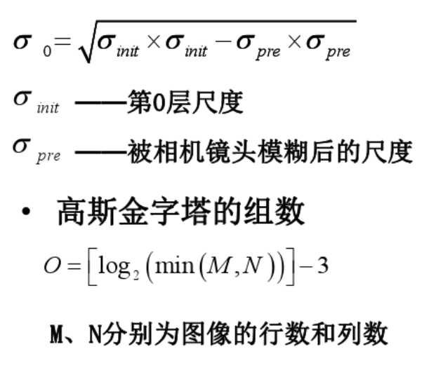
高斯金字塔的初始尺度
当图像通过相机拍摄时,相机的镜头已经对图像进行了一次初始的模糊,所以根据高斯模糊的性质:
下图为构建高斯金字塔的细节图:(图中是从第一层开始算起,其实是一样的)
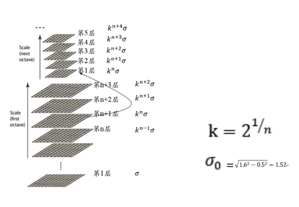
S=n+3 S为每组的总层数,由于上一组第一层由下一组倒数第三层降采样而来,二者高斯尺度相同,将k=2^(1/n)带入可知相邻两组的相同层尺度为2倍的关系。这样可以保持尺度的连续性。
构建DoG金字塔
构建高斯金字塔之后,就是用金字塔相邻图像相减构造DoG金字塔。
下面为构造DoG的代码:
void SIFT::buildDoGPyramid( const vector<Mat>& gpyr, vector<Mat>& dogpyr ) const
{
//计算金字塔的组的数量
    int nOctaves = (int)gpyr.size()/(nOctaveLayers + 3);
 //定义DoG 金字塔的总层数,DoG 金字塔比高斯金字塔每组少一层
    dogpyr.resize( nOctaves*(nOctaveLayers + 2) );
//遍历DoG 的所有层,构建DoG 金字塔
    for( int o = 0; o < nOctaves; o++ )
    {
        for( int i = 0; i < nOctaveLayers + 2; i++ )
        {
        //提取出高斯金字塔的当前层图像
            const Mat& src1 = gpyr[o*(nOctaveLayers + 3) + i];
       //提取出高斯金字塔的上层图像
            const Mat& src2 = gpyr[o*(nOctaveLayers + 3) + i + 1];
       //提取出DoG 金字塔的当前层图像
            Mat& dst = dogpyr[o*(nOctaveLayers + 2) + i];
       //DoG 金字塔的当前层图像等于高斯金字塔的当前层图像减去高斯金字塔的上层图像
            subtract(src2, src1, dst, noArray(), DataType<sift_wt>::type);
        }
    }
由前一步,我们得到了DoG高斯差分金字塔:
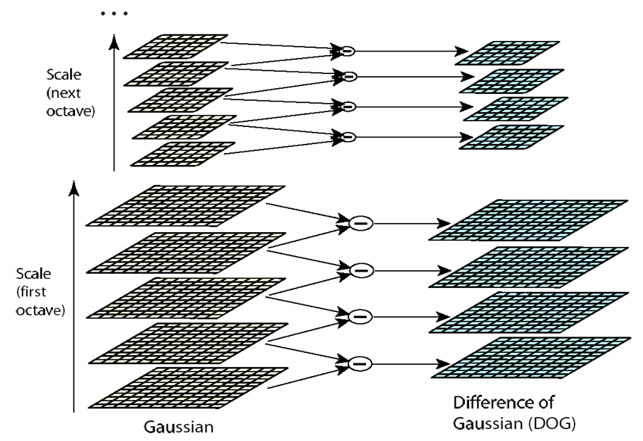
图1
如上图的金字塔,高斯尺度空间金字塔中每组有五层不同尺度图像,相邻两层相减得到四层DoG结果。关键点搜索就在这四层DoG图像上寻找局部极值点。
空间极值点检测(关键点的初步探查)
关键点是由DOG空间的局部极值点组成的,关键点的初步探查是通过同一组内各DoG相邻两层图像之间比较完成的。为了寻找DoG函数的极值点,每一个像素点要和它所有的相邻点比较,看其是否比它的图像域和尺度域的相邻点大或者小。如图3.4所示,中间的检测点和它同尺度的8个相邻点和上下相邻尺度对应的9×2个点共26个点比较,以确保在尺度空间和二维图像空间都检测到极值点。
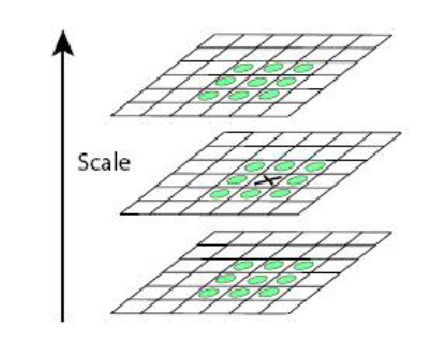
由于要在相邻尺度进行比较,如图1右侧每组含4层的高斯差分金子塔,只能在中间两层中进行两个尺度的极值点检测,其它尺度则只能在不同组中进行。为了在每组中检测S个尺度的极值点,则DOG金字塔每组需S+2层图像,而DOG金字塔由高斯金字塔相邻两层相减得到,则高斯金字塔每组需S+3层图像,实际计算时S在3到5之间。
当然这样产生的极值点并不全都是稳定的特征点,因为某些极值点响应较弱,而且DOG算子会产生较强的边缘响应。
以上方法检测到的极值点是离散空间的极值点,以下通过拟合三维二次函数来精确确定关键点的位置和尺度,同时去除低对比度的关键点和不稳定的边缘响应点(因为DoG算子会产生较强的边缘响应),以增强匹配稳定性、提高抗噪声能力。
关键点的精确定位
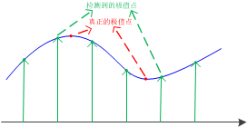
以上极值点的搜索是在离散空间进行搜索的,由下图可以看到,在离散空间找到的极值点不一定是真正意义上的极值点。可以通过对尺度空间DoG函数进行曲线拟合寻找极值点来减小这种误差。
为了提高关键点的稳定性,需要对尺度空间DoG函数进行曲线拟合。利用DoG函数在尺度空间的Taylor展开式(拟合函数)为:
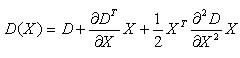
其中, 。求导并让方程等于零,可以得到极值点的偏移量为:
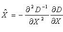
对应极值点,方程的值为:
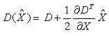
其中, 代表相对插值中心的偏移量,当它在任一维度上的偏移量大于0.5时(即x或y或
 ),意味着插值中心已经偏移到它的邻近点上,所以必须改变当前关键点的位置。同时在新的位置上反复插值直到收敛;也有可能超出所设定的迭代次数或者超出图像边界的范围,此时这样的点应该删除,在Lowe中进行了5次迭代。另外,
 过小的点易受噪声的干扰而变得不稳定,所以将小于某个经验值(Lowe论文中使用0.03,Rob Hess等人实现时使用0.04/S)的极值点删除。同时,在此过程中获取特征点的精确位置(原位置加上拟合的偏移量)以及尺度。
在DoG尺度空间中找极值点,并按照主曲率的对比度删除不好的极值点:


void SIFT::findScaleSpaceExtrema( const vector<Mat>& gauss_pyr, const vector<Mat>& dog_pyr,
                                  vector<KeyPoint>& keypoints ) const
{
//得到金字塔的组数
    int nOctaves = (int)gauss_pyr.size()/(nOctaveLayers + 3);
//SIFT_FIXPT_SCALE = 1,设定一个阈值用于判断在DoG 尺度图像中像素的大小
    int threshold = cvFloor(0.5 * contrastThreshold / nOctaveLayers * 255 * SIFT_FIXPT_SCALE);
//SIFT_ORI_HIST_BINS = 36,定义梯度方向直方图的柱的数量
    const int n = SIFT_ORI_HIST_BINS;
//定义梯度方向直方图变量
    float hist[n];
    KeyPoint kpt;

    keypoints.clear();//清空

    for( int o = 0; o < nOctaves; o++ )
        for( int i = 1; i <= nOctaveLayers; i++ )
        {
        //DoG 金字塔的当前层索引
            int idx = o*(nOctaveLayers+2)+i;
        //DoG 金字塔当前层的尺度图像
            const Mat& img = dog_pyr[idx];
       //DoG 金字塔下层的尺度图像
            const Mat& prev = dog_pyr[idx-1];
       //DoG 金字塔上层的尺度图像
            const Mat& next = dog_pyr[idx+1];

            int step = (int)img.step1();
       //图像的长和宽
            int rows = img.rows, cols = img.cols;
   //SIFT_IMG_BORDER = 5,该变量的作用是保留一部分图像的四周边界
            for( int r = SIFT_IMG_BORDER; r < rows-SIFT_IMG_BORDER; r++)
            {
            //DoG 金字塔当前层图像的当前行指针
                const sift_wt* currptr = img.ptr<sift_wt>(r);
              //DoG 金字塔下层图像的当前行指针
                const sift_wt* prevptr = prev.ptr<sift_wt>(r);
                //DoG 金字塔上层图像的当前行指针
                const sift_wt* nextptr = next.ptr<sift_wt>(r);

                for( int c = SIFT_IMG_BORDER; c < cols-SIFT_IMG_BORDER; c++)
                {
                //DoG 金字塔当前层尺度图像的像素值
                    sift_wt val = currptr[c];

    // find local extrema with pixel accuracy
   //精确定位局部极值点
//如果满足if 条件,则找到了极值点,即候选特征点
                    if( std::abs(val) > threshold &&
 //像素值要大于一定的阈值才稳定,即要具有较强的对比度
//下面的逻辑判断被“与”分为两个部分,前一个部分要满足像素值大于0,在3×3×3 的立方体内与周围26 个邻近像素比较找极大值,
//后一个部分要满足像素值小于0,找极小值
                       ((val > 0 && val >= currptr[c-1] && val >= currptr[c+1] &&
                         val >= currptr[c-step-1] && val >= currptr[c-step] && val >= currptr[c-step+1] &&
                         val >= currptr[c+step-1] && val >= currptr[c+step] && val >= currptr[c+step+1] &&
                         val >= nextptr[c] && val >= nextptr[c-1] && val >= nextptr[c+1] &&
                         val >= nextptr[c-step-1] && val >= nextptr[c-step] && val >= nextptr[c-step+1] &&
                         val >= nextptr[c+step-1] && val >= nextptr[c+step] && val >= nextptr[c+step+1] &&
                         val >= prevptr[c] && val >= prevptr[c-1] && val >= prevptr[c+1] &&
                         val >= prevptr[c-step-1] && val >= prevptr[c-step] && val >= prevptr[c-step+1] &&
                         val >= prevptr[c+step-1] && val >= prevptr[c+step] && val >= prevptr[c+step+1]) ||
                        (val < 0 && val <= currptr[c-1] && val <= currptr[c+1] &&
                         val <= currptr[c-step-1] && val <= currptr[c-step] && val <= currptr[c-step+1] &&
                         val <= currptr[c+step-1] && val <= currptr[c+step] && val <= currptr[c+step+1] &&
                         val <= nextptr[c] && val <= nextptr[c-1] && val <= nextptr[c+1] &&
                         val <= nextptr[c-step-1] && val <= nextptr[c-step] && val <= nextptr[c-step+1] &&
                         val <= nextptr[c+step-1] && val <= nextptr[c+step] && val <= nextptr[c+step+1] &&
                         val <= prevptr[c] && val <= prevptr[c-1] && val <= prevptr[c+1] &&
                         val <= prevptr[c-step-1] && val <= prevptr[c-step] && val <= prevptr[c-step+1] &&
                         val <= prevptr[c+step-1] && val <= prevptr[c+step] && val <= prevptr[c+step+1])))
                    {
    //三维坐标,长、宽、层(层与尺度相对应)
                        int r1 = r, c1 = c, layer = i;
 // adjustLocalExtrema 函数的作用是调整局部极值的位置,即找到亚像素级精度的特征点,该函数在后面给出详细的分析
//如果满足if 条件,说明该极值点不是特征点,继续上面的for循环
                        if( !adjustLocalExtrema(dog_pyr, kpt, o, layer, r1, c1,
                                                nOctaveLayers, (float)contrastThreshold,
                                                (float)edgeThreshold, (float)sigma) )
                            continue;
  //计算特征点相对于它所在组的基准层的尺度,即公式5 所得尺度
                        float scl_octv = kpt.size*0.5f/(1 << o);
// calcOrientationHist 函数为计算特征点的方向角度,后面给出该
函数的详细分析
//SIFT_ORI_SIG_FCTR = 1.5f , SIFT_ORI_RADIUS = 3 *
SIFT_ORI_SIG_FCTR
                        float omax = calcOrientationHist(gauss_pyr[o*(nOctaveLayers+3) + layer],
                                                         Point(c1, r1),
                                                         cvRound(SIFT_ORI_RADIUS * scl_octv),
                                                         SIFT_ORI_SIG_FCTR * scl_octv,
                                                         hist, n);
                                                         //SIFT_ORI_PEAK_RATIO = 0.8f
//计算直方图辅方向的阈值,即主方向的80%
                        float mag_thr = (float)(omax * SIFT_ORI_PEAK_RATIO);
 //计算特征点的方向
                        for( int j = 0; j < n; j++ )
                        {
//j 为直方图当前柱体索引,l 为前一个柱体索引,r2 为后一个柱体索引,如果l 和r2 超出了柱体范围,则要进行圆周循环处理
                            int l = j > 0 ? j - 1 : n - 1;
                            int r2 = j < n-1 ? j + 1 : 0;
//方向角度拟合处理
//判断柱体高度是否大于直方图辅方向的阈值,因为拟合处理的需要,还要满足柱体的高度大于其前后相邻两个柱体的高度
                            if( hist[j] > hist[l]  &&  hist[j] > hist[r2]  &&  hist[j] >= mag_thr )
                            {
                            //公式26
                                float bin = j + 0.5f * (hist[l]-hist[r2]) / (hist[l] - 2*hist[j] + hist[r2]);
                                //圆周循环处理
                                bin = bin < 0 ? n + bin : bin >= n ? bin - n : bin;
                                //公式27,得到特征点的方向
                                kpt.angle = 360.f - (float)((360.f/n) * bin);
              //如果方向角度十分接近于360 度,则就让它等于0 度
                                if(std::abs(kpt.angle - 360.f) < FLT_EPSILON)
                                    kpt.angle = 0.f;
                                //保存特征点
                                keypoints.push_back(kpt);
                            }
                        }
                    }
                }
            }
        }
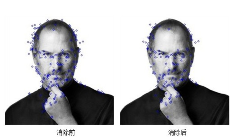
消除边缘响应
仅仅去除低对比度的极值点对于特征点的稳定性是远远不够的。DOG函数在图像边缘有较强的边缘响应,因此我们还需要排除边缘响应。
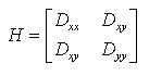
DOG函数的(欠佳的)峰值点在横跨边缘的方向有较大的主曲率,而在垂直边缘的方向有较小的主曲率。主曲率可以通过计算在该点位置尺度的
2×2的Hessian矩阵得到,导数由采样点相邻差来估计:
![]() 表示DOG金字塔中某一尺度的图像x方向求导两次。
表示DOG金字塔中某一尺度的图像x方向求导两次。
H的特征值α和β代表x和y方向的梯度。
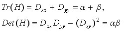
表示矩阵H对角线元素之和,表示矩阵H的行列式。假设是α较大的特征值,而是β较小的特征值,令 ,则
,则
导数由采样点相邻差估计得到,在下一节中说明。
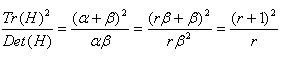
D的主曲率和H的特征值成正比,令为α最大特征值,β为最小的特征值,则公式 的值在两个特征值相等时最小,随着的增大而增大。值越大,说明两个特征值的比值越大,即在某一个方向的梯度值越大,而在另一个方向的梯度值越小,而边缘恰恰就是这种情况。所以为了剔除边缘响应点,需要让该比值小于一定的阈值,因此,为了检测主曲率是否在某域值r下,只需检测
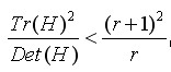
上式成立时将关键点保留,反之剔除。
在Lowe的文章中,取r=10。图4.2右侧为消除边缘响应后的关键点分布图。
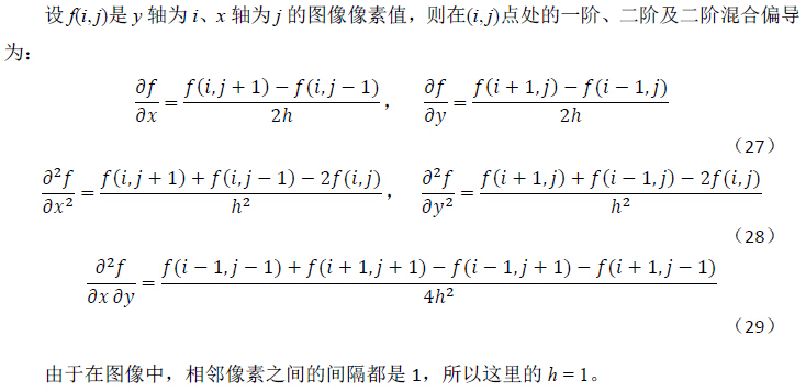
为了求公式15采用的有限差分的式子:
精确找到图像的特征点
//dog_pyr 为DoG 金字塔,kpt 为特征点,octv 和layer 为极值点所在的组和组内的层,r 和c 为极值点的位置坐标
static bool adjustLocalExtrema( const vector<Mat>& dog_pyr, KeyPoint& kpt, int octv,
                                int& layer, int& r, int& c, int nOctaveLayers,
                                float contrastThreshold, float edgeThreshold, float sigma )
{
// SIFT_FIXPT_SCALE = 1,img_scale 为对图像进行归一化处理的系数
    const float img_scale = 1.f/(255*SIFT_FIXPT_SCALE);
    //上面图片中27分母的倒数;
    const float deriv_scale = img_scale*0.5f;
    //上面图片中28分母的倒数;
    const float second_deriv_scale = img_scale;
    //上面图片中29分母的倒数;
    const float cross_deriv_scale = img_scale*0.25f;

    float xi=0, xr=0, xc=0, contr=0;
    int i = 0;
// SIFT_MAX_INTERP_STEPS = 5,表示循环迭代5 次
    for( ; i < SIFT_MAX_INTERP_STEPS; i++ )
    {
    //找到极值点所在的DoG 金字塔的层索引
        int idx = octv*(nOctaveLayers+2) + layer;
        const Mat& img = dog_pyr[idx];//当前层尺度图像
        const Mat& prev = dog_pyr[idx-1];//下层尺度图像
        const Mat& next = dog_pyr[idx+1];//上层尺度图像
//变量dD 就是公式12 中的∂f / ∂X,一阶偏导的公式如上图中27
        Vec3f dD((img.at<sift_wt>(r, c+1) - img.at<sift_wt>(r, c-1))*deriv_scale,//f 对x 的一阶偏导
                 (img.at<sift_wt>(r+1, c) - img.at<sift_wt>(r-1, c))*deriv_scale,//f 对y 的一阶偏导
                 (next.at<sift_wt>(r, c) - prev.at<sift_wt>(r, c))*deriv_scale);//f 对尺度σ的一阶偏导
//当前像素值的2 倍

        float v2 = (float)img.at<sift_wt>(r, c)*2;
 //下面是求二阶纯偏导,如上图中28
//这里的x,y,s 分别代表X = (x, y, σ)T 中的x,y,σ
        float dxx = (img.at<sift_wt>(r, c+1) + img.at<sift_wt>(r, c-1) - v2)*second_deriv_scale;
        float dyy = (img.at<sift_wt>(r+1, c) + img.at<sift_wt>(r-1, c) - v2)*second_deriv_scale;
        float dss = (next.at<sift_wt>(r, c) + prev.at<sift_wt>(r, c) - v2)*second_deriv_scale;
        //下面是求二阶混合偏导,如上图中29
        float dxy = (img.at<sift_wt>(r+1, c+1) - img.at<sift_wt>(r+1, c-1) -
                     img.at<sift_wt>(r-1, c+1) + img.at<sift_wt>(r-1, c-1))*cross_deriv_scale;
        float dxs = (next.at<sift_wt>(r, c+1) - next.at<sift_wt>(r, c-1) -
                     prev.at<sift_wt>(r, c+1) + prev.at<sift_wt>(r, c-1))*cross_deriv_scale;
        float dys = (next.at<sift_wt>(r+1, c) - next.at<sift_wt>(r-1, c) -
                     prev.at<sift_wt>(r+1, c) + prev.at<sift_wt>(r-1, c))*cross_deriv_scale;
//变量H 就是公式8 中的∂2f / ∂X2,它的具体展开形式可以在公式9 中看到
        Matx33f H(dxx, dxy, dxs,
                  dxy, dyy, dys,
                  dxs, dys, dss);
//求方程A×X=B,即X=(A^-1)×B,这里A 就是H,B 就是dD
        Vec3f X = H.solve(dD, DECOMP_LU);
//可以看出上面求得的X 与公式12 求得的变量差了一个符号,因此下面的变量都加上了负号
        xi = -X[2];//层坐标的偏移量,这里的层与图像尺度相对应
        xr = -X[1];//纵坐标的偏移量
        xc = -X[0];//横坐标的偏移量
//如果由泰勒级数插值得到的三个坐标的偏移量都小于0.5,说明已经找到特征点,则退出迭代

        if( std::abs(xi) < 0.5f && std::abs(xr) < 0.5f && std::abs(xc) < 0.5f )
            break;
//如果三个坐标偏移量中任意一个大于一个很大的数,则说明该极值点不是特征点,函数返回
        if( std::abs(xi) > (float)(INT_MAX/3) ||
            std::abs(xr) > (float)(INT_MAX/3) ||
            std::abs(xc) > (float)(INT_MAX/3) )
            return false;//没有找到特征点,返回
//由上面得到的偏移量重新定义插值中心的坐标位置

        c += cvRound(xc);
        r += cvRound(xr);
        layer += cvRound(xi);
//如果新的坐标超出了金字塔的坐标范围,则说明该极值点不是特征点,函数返回
        if( layer < 1 || layer > nOctaveLayers ||
            c < SIFT_IMG_BORDER || c >= img.cols - SIFT_IMG_BORDER  ||
            r < SIFT_IMG_BORDER || r >= img.rows - SIFT_IMG_BORDER )
            return false;//没有找到特征点,返回
    }

    // ensure convergence of interpolation
    //进一步确认是否大于迭代次数
    if( i >= SIFT_MAX_INTERP_STEPS )
        return false;//没有找到特征点,返回

    {
    //由上面得到的层坐标计算它在DoG 金字塔中的层索引
        int idx = octv*(nOctaveLayers+2) + layer;
        //该层索引所对应的DoG 金字塔的当前层尺度图像
        const Mat& img = dog_pyr[idx];
        //DoG 金字塔的下层尺度图像
        const Mat& prev = dog_pyr[idx-1];
        //DoG 金字塔的上层尺度图像
        const Mat& next = dog_pyr[idx+1];
        //再次计算公式12 中的∂f / ∂X
        Matx31f dD((img.at<sift_wt>(r, c+1) - img.at<sift_wt>(r, c-1))*deriv_scale,
                   (img.at<sift_wt>(r+1, c) - img.at<sift_wt>(r-1, c))*deriv_scale,
                   (next.at<sift_wt>(r, c) - prev.at<sift_wt>(r, c))*deriv_scale);
   //dD 点乘(xc, xr, xi),点乘类似于MATLAB 中的点乘
//变量t 就是公式13 中等号右边的第2 项内容
        float t = dD.dot(Matx31f(xc, xr, xi));
//计算公式13,求极值点处图像的灰度值,即响应值
        contr = img.at<sift_wt>(r, c)*img_scale + t * 0.5f;
        //由公式14 判断响应值是否稳定
        if( std::abs( contr ) * nOctaveLayers < contrastThreshold )
            return false;//不稳定的极值,说明没有找到特征点,返回

        // principal curvatures are computed using the trace and det of Hessian
        //边缘极值点的判断
        float v2 = img.at<sift_wt>(r, c)*2.f;//当前像素灰度值的2 倍
        //计算矩阵H 的4 个元素
//二阶纯偏导,如上图中的28
        float dxx = (img.at<sift_wt>(r, c+1) + img.at<sift_wt>(r, c-1) - v2)*second_deriv_scale;
        float dyy = (img.at<sift_wt>(r+1, c) + img.at<sift_wt>(r-1, c) - v2)*second_deriv_scale;
        //二阶混合偏导,如上图29
        float dxy = (img.at<sift_wt>(r+1, c+1) - img.at<sift_wt>(r+1, c-1) -
                     img.at<sift_wt>(r-1, c+1) + img.at<sift_wt>(r-1, c-1)) * cross_deriv_scale;
       //求矩阵的直迹,公式16
        float tr = dxx + dyy;
        //求矩阵的行列式,公式17
        float det = dxx * dyy - dxy * dxy;
//逻辑“或”的前一项表示矩阵的行列式值不能小于0,后一项如公式19
        if( det <= 0 || tr*tr*edgeThreshold >= (edgeThreshold + 1)*(edgeThreshold + 1)*det )
            return false;//不是特征点,返回
    }
//保存特征点信息
//特征点对应于输入图像的横坐标位置
    kpt.pt.x = (c + xc) * (1 << octv);
    //特征点对应于输入图像的纵坐标位置
//需要注意的是,这里的输入图像特指实际的输入图像扩大一倍以后的图像,因为这里的octv 是包括了前面理论分析部分提到的金字塔
//的第‐1 组
    kpt.pt.y = (r + xr) * (1 << octv);
    //按一定格式保存特征点所在的组、层以及插值后的层的偏移量
    kpt.octave = octv + (layer << 8) + (cvRound((xi + 0.5)*255) << 16);
    //特征点相对于输入图像的尺度,即公式5
//同样的,这里的输入图像也是特指实际的输入图像扩大一倍以后的图像,所以下面的语句其实是比公式5 多了一项——乘以2
    kpt.size = sigma*powf(2.f, (layer + xi) / nOctaveLayers)*(1 << octv)*2;
    //特征点的响应值
    kpt.response = std::abs(contr);
//是特征点,返回
    return true;
我们已经找到了关键点。为了实现图像旋转不变性,需要根据检测到的关键点局部图像结构为特征点方向赋值。也就是在findScaleSpaceExtrema()函数里看到的alcOrientationHist()语句:
我们使用图像的梯度直方图法求关键点局部结构的稳定方向。
梯度方向和幅值
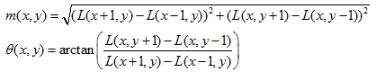
在前文中,精确定位关键点后也找到改特征点的尺度值σ,根据这一尺度值,得到最接近这一尺度值的高斯图像:
使用有限差分,计算以关键点为中心,以3×1.5σ为半径的区域内图像梯度的幅角和幅值,公式如下:
梯度直方图
在完成关键点邻域内高斯图像梯度计算后,使用直方图统计邻域内像素对应的梯度方向和幅值。
有关直方图的基础知识可以参考《数字图像直方图》,可以看做是离散点的概率表示形式。此处方向直方图的核心是统计以关键点为原点,一定区域内的图像像素点对关键点方向生成所作的贡献。
梯度方向直方图的横轴是梯度方向角,纵轴是剃度方向角对应的梯度幅值累加值。梯度方向直方图将0°~360°的范围分为36个柱,每10°为一个柱。下图是从高斯图像上求取梯度,再由梯度得到梯度方向直方图的例图。
在计算直方图时,每个加入直方图的采样点都使用圆形高斯函数函数进行了加权处理,也就是进行高斯平滑。这主要是因为SIFT算法只考虑了尺度和旋转不变形,没有考虑仿射不变性。通过高斯平滑,可以使关键点附近的梯度幅值有较大权重,从而部分弥补没考虑仿射不变形产生的特征点不稳定。
通常离散的梯度直方图要进行插值拟合处理,以求取更精确的方向角度值。(这和《关键点搜索与定位》中插值的思路是一样的)。
关键点方向
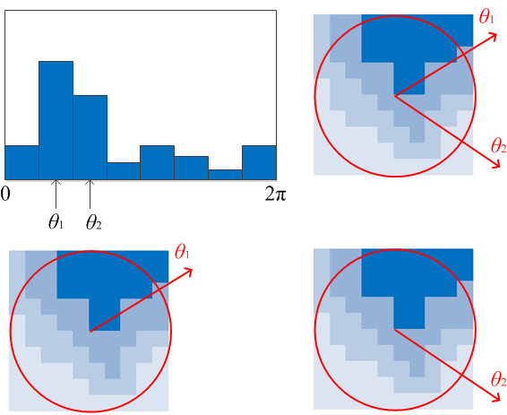
直方图峰值代表该关键点处邻域内图像梯度的主方向,也就是该关键点的主方向。在梯度方向直方图中,当存在另一个相当于主峰值 80%能量的峰值时,则将这个方向认为是该关键点的辅方向。所以一个关键点可能检测得到多个方向,这可以增强匹配的鲁棒性。Lowe的论文指出大概有15%关键点具有多方向,但这些点对匹配的稳定性至为关键。
获得图像关键点主方向后,每个关键点有三个信息(x,y,σ,θ):位置、尺度、方向。由此我们可以确定一个SIFT特征区域。通常使用一个带箭头的圆或直接使用箭头表示SIFT区域的三个值:中心表示特征点位置,半径表示关键点尺度(r=2.5σ),箭头表示主方向。具有多个方向的关键点可以复制成多份,然后将方向值分别赋给复制后的关键点。如下图:
计算特征点的方向角度
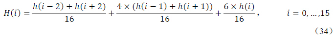
上图是opencv中使用的方向直方图的平滑公式,与lowe推荐的不同
// Computes a gradient orientation histogram at a specified pixel
//img 为特征点所在的高斯尺度图像;
//pt 为特征点在该尺度图像的坐标点;
//radius 为邻域半径,即公式30;
//sigma 为高斯函数的方差,即公式33;
//hist 为梯度方向直方图;
//n 为梯度方向直方图柱体的数量,n=36
//该函数返回直方图的主峰值
static float calcOrientationHist( const Mat& img, Point pt, int radius,
                                  float sigma, float* hist, int n )
{
//len 为计算特征点方向时的特征点领域像素的数量
    int i, j, k, len = (radius*2+1)*(radius*2+1);
// expf_scale 为高斯加权函数中e 指数中的常数部分
    float expf_scale = -1.f/(2.f * sigma * sigma);
    //分配一段内存空间
//X 表示x 轴方向的差分,Y 表示y 轴方向的差分,Mag 为梯度幅值,Ori 为梯度幅角,W 为高斯加权值
//上述变量在buf 空间的分配是:X 和Mag 共享一段长度为len 的空间,Y 和Ori 分别占用一段长度为len 的空间,W 占用一段
//长度为len+2 的空间,它们的空间顺序为X(Mag)在buf 的最下面,然后是Y,Ori,最后是W
    float *X = buf, *Y = X + len, *Mag = X, *Ori = Y + len, *W = Ori + len;
    //temphist 表示暂存的梯度方向直方图,空间长度为n+2,空间位置是在W 的上面
//之所以temphist 的长度是n+2,W 的长度是len+2,而不是n 和len,是因为要进行圆周循环操作,必须给temphist 的前后各
//留出两个空间位置
    float* temphist = W + len + 2;

    for( i = 0; i < n; i++ )
    //直方图变量清空
        temphist[i] = 0.f;
//计算x 轴、y 轴方向的导数,以及高斯加权值
    for( i = -radius, k = 0; i <= radius; i++ )
    {
        int y = pt.y + i;//邻域像素的y 轴坐标
//判断y 轴坐标是否超出图像的范围
        if( y <= 0 || y >= img.rows - 1 )
            continue;
        for( j = -radius; j <= radius; j++ )
        {
            int x = pt.x + j;//邻域像素的x 轴坐标
//判断x 轴坐标是否超出图像的范围
            if( x <= 0 || x >= img.cols - 1 )
                continue;
//分别计算x 轴和y 轴方向的差分,即上图中27 的分子部分,因为只需要相对
值,所有分母部分可以不用计算
            float dx = (float)(img.at<sift_wt>(y, x+1) - img.at<sift_wt>(y, x-1));
            float dy = (float)(img.at<sift_wt>(y-1, x) - img.at<sift_wt>(y+1, x));
//保存变量,这里的W 为高斯函数的e 指数
            X[k] = dx; Y[k] = dy; W[k] = (i*i + j*j)*expf_scale;
            k++;//邻域像素的计数值加1
        }
    }
//这里的len 为特征点实际的邻域像素的数量
    len = k;

    // compute gradient values, orientations and the weights over the pixel neighborhood
    //计算邻域中所有元素的高斯加权值W,梯度幅角Ori 和梯度幅值Mag
    exp(W, W, len);
    fastAtan2(Y, X, Ori, len, true);
    magnitude(X, Y, Mag, len);
//计算梯度方向直方图
    for( k = 0; k < len; k++ )
    {
    //判断邻域像素的梯度幅角属于36 个柱体的哪一个
        int bin = cvRound((n/360.f)*Ori[k]);
        //如果超出范围,则利用圆周循环确定其真正属于的那个柱体
        if( bin >= n )
            bin -= n;
        if( bin < 0 )
            bin += n;
            //累积经高斯加权处理后的梯度幅值
        temphist[bin] += W[k]*Mag[k];
    }

    // smooth the histogram
    //平滑直方图
//为了圆周循环,提前填充好直方图前后各两个变量
    temphist[-1] = temphist[n-1];
    temphist[-2] = temphist[n-2];
    temphist[n] = temphist[0];
    temphist[n+1] = temphist[1];
    for( i = 0; i < n; i++ )
    {
    //利用上图中公式34,进行平滑直方图操作,注意这里与lowe建议的方法不一样
        hist[i] = (temphist[i-2] + temphist[i+2])*(1.f/16.f) +
            (temphist[i-1] + temphist[i+1])*(4.f/16.f) +
            temphist[i]*(6.f/16.f);
    }
//计算直方图的主峰值
    float maxval = hist[0];
    for( i = 1; i < n; i++ )
        maxval = std::max(maxval, hist[i]);

    return maxval;//返回直方图的主峰值
}
为找到的关键点即SIFT特征点赋了值,包含位置、尺度和方向的信息。接下来的步骤是关键点描述,特征描述的目的是在关键点计算后,用一组向量将这个关键点描述出来,这个描述子不但包括关键点,也包括关键点周围对其有贡献的像素点。用来作为目标匹配的依据(所以描述子应该有较高的独特性,以保证匹配率),也可使关键点具有更多的不变特性,如光照变化、3D视点变化等。
SIFT描述子h(x,y,θ)是对关键点附近邻域内高斯图像梯度统计的结果,是一个三维矩阵,但通常用一个矢量来表示。矢量通过对三维矩阵按一定规律排列得到。
描述子采样区域
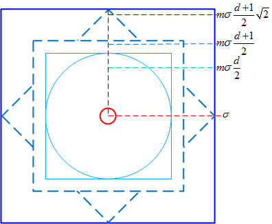
特征描述子与关键点所在尺度有关,因此对梯度的求取应在特征点对应的高斯图像上进行。将关键点附近划分成d×d个子区域,每个子区域尺寸为mσ个像元(d=4,m=3,σ为尺特征点的尺度值)。考虑到实际计算时需要双线性插值,故计算的图像区域为mσ(d+1),再考虑旋转,则实际计算的图像区域为,如下图所示:
源码
 Point pt(cvRound(ptf.x), cvRound(ptf.y));
    //计算余弦,正弦,CV_PI/180:将角度值转化为幅度值
    float cos_t = cosf(ori*(float)(CV_PI/180));
    float sin_t = sinf(ori*(float)(CV_PI/180));
    float bins_per_rad = n / 360.f;
    float exp_scale = -1.f/(d * d * 0.5f); //d:SIFT_DESCR_WIDTH 4
    float hist_width = SIFT_DESCR_SCL_FCTR * scl;  // SIFT_DESCR_SCL_FCTR: 3
                                                   // scl: size*0.5f
    // 计算图像区域半径mσ(d+1)/2*sqrt(2)
    // 1.4142135623730951f 为根号2
    int radius = cvRound(hist_width * 1.4142135623730951f * (d + 1) * 0.5f);
    cos_t /= hist_width;
    sin_t /= hist_width;
区域坐标轴旋转
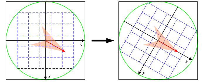
旋转后区域内采样点新的坐标为:
源码
//计算采样区域点坐标旋转
    for( i = -radius, k = 0; i <= radius; i++ )
        for( j = -radius; j <= radius; j++ )
        {
            /*
             Calculate sample's histogram array coords rotated relative to ori.
             Subtract 0.5 so samples that fall e.g. in the center of row 1 (i.e.
             r_rot = 1.5) have full weight placed in row 1 after interpolation.
             */
            float c_rot = j * cos_t - i * sin_t;
            float r_rot = j * sin_t + i * cos_t;
            float rbin = r_rot + d/2 - 0.5f;
            float cbin = c_rot + d/2 - 0.5f;
            int r = pt.y + i, c = pt.x + j;

            if( rbin > -1 && rbin < d && cbin > -1 && cbin < d &&
               r > 0 && r < rows - 1 && c > 0 && c < cols - 1 )
            {
                float dx = (float)(img.at<short>(r, c+1) - img.at<short>(r, c-1));
                float dy = (float)(img.at<short>(r-1, c) - img.at<short>(r+1, c));
                X[k] = dx; Y[k] = dy; RBin[k] = rbin; CBin[k] = cbin;
                W[k] = (c_rot * c_rot + r_rot * r_rot)*exp_scale;
                k++;
            }
        }
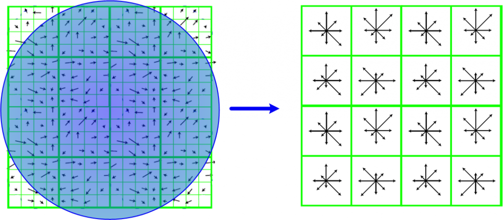
计算采样区域梯度直方图
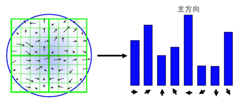
将旋转后区域划分为d×d个子区域(每个区域间隔为mσ像元),在子区域内计算8个方向的梯度直方图,绘制每个方向梯度方向的累加值,形成一个种子点。
与求主方向不同的是,此时,每个子区域梯度方向直方图将0°~360°划分为8个方向区间,每个区间为45°。即每个种子点有8个方向区间的梯度强度信息。由于存在d×d,即4×4个子区域,所以最终共有4×4×8=128个数据,形成128维SIFT特征矢量。
源码
static void calcSIFTDescriptor( const Mat& img, Point2f ptf, float ori, float scl,
                               int d, int n, float* dst )
{
    Point pt(cvRound(ptf.x), cvRound(ptf.y));//特征点的位置坐标
//特征点方向的余弦和正弦,即cosθ 和sinθ
    float cos_t = cosf(ori*(float)(CV_PI/180));
    float sin_t = sinf(ori*(float)(CV_PI/180));
    //n = 8,45 度的倒数
    float bins_per_rad = n / 360.f;
    //高斯加权函数中的e 指数的常数部分
    float exp_scale = -1.f/(d * d * 0.5f);
    //SIFT_DESCR_SCL_FCTR = 3.f,即3σ
    float hist_width = SIFT_DESCR_SCL_FCTR * scl;
    //特征点邻域区域的半径,即公式28
    int radius = cvRound(hist_width * 1.4142135623730951f * (d + 1) * 0.5f);
    // Clip the radius to the diagonal of the image to avoid autobuffer too large exception
    //避免邻域过大
    radius = std::min(radius, (int) sqrt((double) img.cols*img.cols + img.rows*img.rows));
    //归一化处理
    cos_t /= hist_width;
    sin_t /= hist_width;
//len 为特征点邻域区域内像素的数量,histlen 为直方图的数量,即特征矢量的长度,实际应为d×d×n,之所以每个变量
//又加上了2,是因为要为圆周循环留出一定的内存空间
    int i, j, k, len = (radius*2+1)*(radius*2+1), histlen = (d+2)*(d+2)*(n+2);
    int rows = img.rows, cols = img.cols;//特征点所在的尺度图像的长和宽
//开辟一段内存空间

    AutoBuffer<float> buf(len*6 + histlen);
    //X 表示x 方向梯度,Y 表示y 方向梯度,Mag 表示梯度幅值,Ori 表示梯度幅角,W 为高斯加权值,其中Y 和Mag
    // 共享一段内存空间,长度都为len,它们在buf 的顺序为X 在最下面,然后是Y(Mag),Ori,最后是W
    float *X = buf, *Y = X + len, *Mag = Y, *Ori = Mag + len, *W = Ori + len;
    //下面是三维直方图的变量,RBin 和CBin 分别表示d×d 邻域范围的横、纵坐标,hist 表示直方图的值。RBin
    //和CBin 的长度都是len,hist 的长度为histlen,顺序为RBin 在W 的上面,然后是CBin,最后是hist
    float *RBin = W + len, *CBin = RBin + len, *hist = CBin + len;
//直方图数组hist 清零
    for( i = 0; i < d+2; i++ )
    {
        for( j = 0; j < d+2; j++ )
            for( k = 0; k < n+2; k++ )
                hist[(i*(d+2) + j)*(n+2) + k] = 0.;
    }
//遍历当前特征点的邻域范围
    for( i = -radius, k = 0; i <= radius; i++ )
        for( j = -radius; j <= radius; j++ )
        {
            // Calculate sample's histogram array coords rotated relative to ori.
            // Subtract 0.5 so samples that fall e.g. in the center of row 1 (i.e.
            // r_rot = 1.5) have full weight placed in row 1 after interpolation.
            //根据公式29 计算旋转后的位置坐标
            float c_rot = j * cos_t - i * sin_t;
            float r_rot = j * sin_t + i * cos_t;
            //把邻域区域的原点从中心位置移到该区域的左下角,以便后面的使用。因为变量cos_t 和sin_t 都已
            //进行了归一化处理,所以原点位移时只需要加d/2 即可。而再减0.5f的目的是进行坐标平移,从而在
            //三线性插值计算中,计算的是正方体内的点对正方体8 个顶点的贡献大小,而不是对正方体的中心点的
            //贡献大小。之所以没有对角度obin 进行坐标平移,是因为角度是连续的量,无需平移
            float rbin = r_rot + d/2 - 0.5f;
            float cbin = c_rot + d/2 - 0.5f;
            //得到邻域像素点的位置坐标
            int r = pt.y + i, c = pt.x + j;
//确定邻域像素是否在d×d 的正方形内,以及是否超过了图像边界
            if( rbin > -1 && rbin < d && cbin > -1 && cbin < d &&
                r > 0 && r < rows - 1 && c > 0 && c < cols - 1 )
            {
            //根据上图中27 计算x 和y 方向的一阶导数,这里省略了公式中的分母部分,因为没有分母部分不影响
            //后面所进行的归一化处理
                float dx = (float)(img.at<sift_wt>(r, c+1) - img.at<sift_wt>(r, c-1));

                float dy = (float)(img.at<sift_wt>(r-1, c) - img.at<sift_wt>(r+1, c));
                //保存到各自的数组中
                X[k] = dx; Y[k] = dy; RBin[k] = rbin; CBin[k] = cbin;
                //高斯加权函数中的e 指数部分
                W[k] = (c_rot * c_rot + r_rot * r_rot)*exp_scale;
                k++;//统计实际的邻域像素的数量
            }
        }

    len = k;//赋值
    fastAtan2(Y, X, Ori, len, true);//计算梯度幅角
    magnitude(X, Y, Mag, len);//计算梯度幅值
    exp(W, W, len);//计算高斯加权函数
//遍历所有邻域像素
    for( k = 0; k < len; k++ )
    {
    //得到d×d 邻域区域的坐标,即三维直方图的底内的位置
        float rbin = RBin[k], cbin = CBin[k];
        //得到幅角所属的8 等份中的某一个等份,即三维直方图的高的位置
        float obin = (Ori[k] - ori)*bins_per_rad;
        float mag = Mag[k]*W[k];//得到高斯加权以后的梯度幅值
//向下取整
//r0,c0 和o0 为三维坐标的整数部分,它表示属于的哪个正方体
        int r0 = cvFloor( rbin );
        int c0 = cvFloor( cbin );
        int o0 = cvFloor( obin );
        //小数部分
//rbin,cbin 和obin 为三维坐标的小数部分,即将中心点移动到正方体端点时C 点在正方体的坐标
        rbin -= r0;
        cbin -= c0;
        obin -= o0;
//如果角度o0 小于0 度或大于360 度,则根据圆周循环,把该角度调整到0~360度之间
        if( o0 < 0 )
            o0 += n;
        if( o0 >= n )
            o0 -= n;

        // histogram update using tri-linear interpolation
        //根据三线性插值法,计算该像素对正方体的8 个顶点的贡献大小,即公式39 中得到的8 个立方体的体积,
        //当然这里还需要乘以高斯加权后的梯度值mag
        float v_r1 = mag*rbin, v_r0 = mag - v_r1;
        float v_rc11 = v_r1*cbin, v_rc10 = v_r1 - v_rc11;
        float v_rc01 = v_r0*cbin, v_rc00 = v_r0 - v_rc01;
        float v_rco111 = v_rc11*obin, v_rco110 = v_rc11 - v_rco111;
        float v_rco101 = v_rc10*obin, v_rco100 = v_rc10 - v_rco101;
        float v_rco011 = v_rc01*obin, v_rco010 = v_rc01 - v_rco011;
        float v_rco001 = v_rc00*obin, v_rco000 = v_rc00 - v_rco001;
//得到该像素点在三维直方图中的索引
        int idx = ((r0+1)*(d+2) + c0+1)*(n+2) + o0;
        //8 个顶点对应于坐标平移前的8 个直方图的正方体,对其进行累加求和
        hist[idx] += v_rco000;
        hist[idx+1] += v_rco001;
        hist[idx+(n+2)] += v_rco010;
        hist[idx+(n+3)] += v_rco011;
        hist[idx+(d+2)*(n+2)] += v_rco100;
        hist[idx+(d+2)*(n+2)+1] += v_rco101;
        hist[idx+(d+3)*(n+2)] += v_rco110;
        hist[idx+(d+3)*(n+2)+1] += v_rco111;
    }

    // finalize histogram, since the orientation histograms are circular
    //由于圆周循环的特性,对计算以后幅角小于0 度或大于360 度的值重新进行调整,使其在0~360 度之间
    for( i = 0; i < d; i++ )
        for( j = 0; j < d; j++ )
        {
            int idx = ((i+1)*(d+2) + (j+1))*(n+2);
            hist[idx] += hist[idx+n];
            hist[idx+1] += hist[idx+n+1];
            for( k = 0; k < n; k++ )
                dst[(i*d + j)*n + k] = hist[idx+k];
        }
    // copy histogram to the descriptor,
    // apply hysteresis thresholding
    // and scale the result, so that it can be easily converted
    // to byte array
    float nrm2 = 0;
    len = d*d*n;//特征矢量的维数——128
    for( k = 0; k < len; k++ )
        nrm2 += dst[k]*dst[k];//平方和
        //为了避免计算中的累加误差,对光照阈值进行反归一化处理,即0.2 乘以公式31 中的分母部分,
        //得到反归一化阈值thr
    float thr = std::sqrt(nrm2)*SIFT_DESCR_MAG_THR;
    for( i = 0, nrm2 = 0; i < k; i++ )
    {
    //把特征矢量中大于反归一化阈值thr 的元素用thr 替代
        float val = std::min(dst[i], thr);
        dst[i] = val;
        nrm2 += val*val;//平方和
    }
    //SIFT_INT_DESCR_FCTR = 512.f,浮点型转换为整型时所用到的系数
//归一化处理,计算公式31 中的分母部分
    nrm2 = SIFT_INT_DESCR_FCTR/std::max(std::sqrt(nrm2), FLT_EPSILON);

#if 1
    for( k = 0; k < len; k++ )
    {
    //最终归一化后的特征矢量
        dst[k] = saturate_cast<uchar>(dst[k]*nrm2);
    }
#else
    float nrm1 = 0;
    for( k = 0; k < len; k++ )
    {
        dst[k] *= nrm2;
        nrm1 += dst[k];
    }
    nrm1 = 1.f/std::max(nrm1, FLT_EPSILON);
    for( k = 0; k < len; k++ )
    {
        dst[k] = std::sqrt(dst[k] * nrm1);//saturate_cast<uchar>(std::sqrt(dst[k] * nrm1)*SIFT_INT_DESCR_FCTR);
    }
#endif
完整代码:
#include "precomp.hpp" #include <iostream> #include <stdarg.h> namespace cv { /*************** 定义会用到的参数和宏 ****************/ // 每一组中默认的采样数,即小s的值。 static const int SIFT_INTVLS = 3; //最初的高斯模糊的尺度默认值,即假设的第0组(某些地方叫做-1组)的尺度 static const float SIFT_SIGMA = 1.6f; // 关键点对比 |D(x)|的默认值,公式14的阈值 static const float SIFT_CONTR_THR = 0.04f; // 关键点的主曲率比的默认阈值 static const float SIFT_CURV_THR = 10.f; //是否在构建高斯金字塔之前扩展图像的宽和高位原来的两倍(即是否建立-1组) static const bool SIFT_IMG_DBL = true; // 描述子直方图数组的默认宽度,即描述子建立中的4*4的周边区域 static const int SIFT_DESCR_WIDTH = 4; // 每个描述子数组中的默认柱的个数( 4*4*8=128) static const int SIFT_DESCR_HIST_BINS = 8; // 假设输入图像的高斯模糊的尺度 static const float SIFT_INIT_SIGMA = 0.5f; // width of border in which to ignore keypoints static const int SIFT_IMG_BORDER = 5; //公式12的为了寻找关键点插值中心的最大迭代次数 static const int SIFT_MAX_INTERP_STEPS = 5; // 方向梯度直方图中的柱的个数 static const int SIFT_ORI_HIST_BINS = 36; // determines gaussian sigma for orientation assignment static const float SIFT_ORI_SIG_FCTR = 1.5f; // determines the radius of the region used in orientation assignment static const float SIFT_ORI_RADIUS = 3 * SIFT_ORI_SIG_FCTR; // orientation magnitude relative to max that results in new feature static const float SIFT_ORI_PEAK_RATIO = 0.8f; // determines the size of a single descriptor orientation histogram static const float SIFT_DESCR_SCL_FCTR = 3.f; // threshold on magnitude of elements of descriptor vector static const float SIFT_DESCR_MAG_THR = 0.2f; // factor used to convert floating-point descriptor to unsigned char static const float SIFT_INT_DESCR_FCTR = 512.f; #if 0 // intermediate type used for DoG pyramids typedef short sift_wt; static const int SIFT_FIXPT_SCALE = 48; #else // intermediate type used for DoG pyramids typedef float sift_wt; static const int SIFT_FIXPT_SCALE = 1; #endif static inline void unpackOctave(const KeyPoint& kpt, int& octave, int& layer, float& scale) { octave = kpt.octave & 255; layer = (kpt.octave >> 8) & 255; octave = octave < 128 ? octave : (-128 | octave); scale = octave >= 0 ? 1.f/(1 << octave) : (float)(1 << -octave); } //1、创建基图像矩阵createInitialImage 函数: static Mat createInitialImage( const Mat& img, bool doubleImageSize, float sigma ) { Mat gray, gray_fpt; if( img.channels() == 3 || img.channels() == 4 ) cvtColor(img, gray, COLOR_BGR2GRAY); else img.copyTo(gray); //typedef float sift_wt; //static const int SIFT_FIXPT_SCALE = 1 gray.convertTo(gray_fpt, DataType<sift_wt>::type, SIFT_FIXPT_SCALE, 0); float sig_diff; if( doubleImageSize ) { sig_diff = sqrtf( std::max(sigma * sigma - SIFT_INIT_SIGMA * SIFT_INIT_SIGMA * 4, 0.01f) ); Mat dbl; resize(gray_fpt, dbl, Size(gray.cols*2, gray.rows*2), 0, 0, INTER_LINEAR); GaussianBlur(dbl, dbl, Size(), sig_diff, sig_diff); return dbl; } else { sig_diff = sqrtf( std::max(sigma * sigma - SIFT_INIT_SIGMA * SIFT_INIT_SIGMA, 0.01f) ); GaussianBlur(gray_fpt, gray_fpt, Size(), sig_diff, sig_diff); return gray_fpt; } } 2、建立高斯金字塔 void SIFT::buildGaussianPyramid( const Mat& base, vector<Mat>& pyr, int nOctaves ) const { vector<double> sig(nOctaveLayers + 3); pyr.resize(nOctaves*(nOctaveLayers + 3)); // precompute Gaussian sigmas using the following formula: // \sigma_{total}^2 = \sigma_{i}^2 + \sigma_{i-1}^2 sig[0] = sigma; double k = pow( 2., 1. / nOctaveLayers ); for( int i = 1; i < nOctaveLayers + 3; i++ ) { double sig_prev = pow(k, (double)(i-1))*sigma; double sig_total = sig_prev*k; sig[i] = std::sqrt(sig_total*sig_total - sig_prev*sig_prev); } for( int o = 0; o < nOctaves; o++ ) { for( int i = 0; i < nOctaveLayers + 3; i++ ) { Mat& dst = pyr[o*(nOctaveLayers + 3) + i]; if( o == 0 && i == 0 ) dst = base; // base of new octave is halved image from end of previous octave else if( i == 0 ) { const Mat& src = pyr[(o-1)*(nOctaveLayers + 3) + nOctaveLayers]; resize(src, dst, Size(src.cols/2, src.rows/2), 0, 0, INTER_NEAREST); } else { const Mat& src = pyr[o*(nOctaveLayers + 3) + i-1]; GaussianBlur(src, dst, Size(), sig[i], sig[i]); } } } } 3、建立DoG金字塔 void SIFT::buildDoGPyramid( const vector<Mat>& gpyr, vector<Mat>& dogpyr ) const { int nOctaves = (int)gpyr.size()/(nOctaveLayers + 3); dogpyr.resize( nOctaves*(nOctaveLayers + 2) ); for( int o = 0; o < nOctaves; o++ ) { for( int i = 0; i < nOctaveLayers + 2; i++ ) { const Mat& src1 = gpyr[o*(nOctaveLayers + 3) + i]; const Mat& src2 = gpyr[o*(nOctaveLayers + 3) + i + 1]; Mat& dst = dogpyr[o*(nOctaveLayers + 2) + i]; subtract(src2, src1, dst, noArray(), DataType<sift_wt>::type); } } } 4、2 建立方向直方图 // Computes a gradient orientation histogram at a specified pixel static float calcOrientationHist( const Mat& img, Point pt, int radius, float sigma, float* hist, int n ) { int i, j, k, len = (radius*2+1)*(radius*2+1); float expf_scale = -1.f/(2.f * sigma * sigma); AutoBuffer<float> buf(len*4 + n+4); float *X = buf, *Y = X + len, *Mag = X, *Ori = Y + len, *W = Ori + len; float* temphist = W + len + 2; for( i = 0; i < n; i++ ) temphist[i] = 0.f; for( i = -radius, k = 0; i <= radius; i++ ) { int y = pt.y + i; if( y <= 0 || y >= img.rows - 1 ) continue; for( j = -radius; j <= radius; j++ ) { int x = pt.x + j; if( x <= 0 || x >= img.cols - 1 ) continue; float dx = (float)(img.at<sift_wt>(y, x+1) - img.at<sift_wt>(y, x-1)); float dy = (float)(img.at<sift_wt>(y-1, x) - img.at<sift_wt>(y+1, x)); X[k] = dx; Y[k] = dy; W[k] = (i*i + j*j)*expf_scale; k++; } } len = k; // compute gradient values, orientations and the weights over the pixel neighborhood exp(W, W, len); fastAtan2(Y, X, Ori, len, true); magnitude(X, Y, Mag, len); for( k = 0; k < len; k++ ) { int bin = cvRound((n/360.f)*Ori[k]); if( bin >= n ) bin -= n; if( bin < 0 ) bin += n; temphist[bin] += W[k]*Mag[k]; } // smooth the histogram temphist[-1] = temphist[n-1]; temphist[-2] = temphist[n-2]; temphist[n] = temphist[0]; temphist[n+1] = temphist[1]; for( i = 0; i < n; i++ ) { hist[i] = (temphist[i-2] + temphist[i+2])*(1.f/16.f) + (temphist[i-1] + temphist[i+1])*(4.f/16.f) + temphist[i]*(6.f/16.f); } float maxval = hist[0]; for( i = 1; i < n; i++ ) maxval = std::max(maxval, hist[i]); return maxval; } 4.1、尺度空间中关键点插值过滤 // // Interpolates a scale-space extremum's location and scale to subpixel // accuracy to form an image feature. Rejects features with low contrast. // Based on Section 4 of Lowe's paper. static bool adjustLocalExtrema( const vector<Mat>& dog_pyr, KeyPoint& kpt, int octv, int& layer, int& r, int& c, int nOctaveLayers, float contrastThreshold, float edgeThreshold, float sigma ) { const float img_scale = 1.f/(255*SIFT_FIXPT_SCALE); const float deriv_scale = img_scale*0.5f; const float second_deriv_scale = img_scale; const float cross_deriv_scale = img_scale*0.25f; float xi=0, xr=0, xc=0, contr=0; int i = 0; for( ; i < SIFT_MAX_INTERP_STEPS; i++ ) { int idx = octv*(nOctaveLayers+2) + layer; const Mat& img = dog_pyr[idx]; const Mat& prev = dog_pyr[idx-1]; const Mat& next = dog_pyr[idx+1]; Vec3f dD((img.at<sift_wt>(r, c+1) - img.at<sift_wt>(r, c-1))*deriv_scale, (img.at<sift_wt>(r+1, c) - img.at<sift_wt>(r-1, c))*deriv_scale, (next.at<sift_wt>(r, c) - prev.at<sift_wt>(r, c))*deriv_scale); float v2 = (float)img.at<sift_wt>(r, c)*2; float dxx = (img.at<sift_wt>(r, c+1) + img.at<sift_wt>(r, c-1) - v2)*second_deriv_scale; float dyy = (img.at<sift_wt>(r+1, c) + img.at<sift_wt>(r-1, c) - v2)*second_deriv_scale; float dss = (next.at<sift_wt>(r, c) + prev.at<sift_wt>(r, c) - v2)*second_deriv_scale; float dxy = (img.at<sift_wt>(r+1, c+1) - img.at<sift_wt>(r+1, c-1) - img.at<sift_wt>(r-1, c+1) + img.at<sift_wt>(r-1, c-1))*cross_deriv_scale; float dxs = (next.at<sift_wt>(r, c+1) - next.at<sift_wt>(r, c-1) - prev.at<sift_wt>(r, c+1) + prev.at<sift_wt>(r, c-1))*cross_deriv_scale; float dys = (next.at<sift_wt>(r+1, c) - next.at<sift_wt>(r-1, c) - prev.at<sift_wt>(r+1, c) + prev.at<sift_wt>(r-1, c))*cross_deriv_scale; Matx33f H(dxx, dxy, dxs, dxy, dyy, dys, dxs, dys, dss); Vec3f X = H.solve(dD, DECOMP_LU); xi = -X[2]; xr = -X[1]; xc = -X[0]; if( std::abs(xi) < 0.5f && std::abs(xr) < 0.5f && std::abs(xc) < 0.5f ) break; if( std::abs(xi) > (float)(INT_MAX/3) || std::abs(xr) > (float)(INT_MAX/3) || std::abs(xc) > (float)(INT_MAX/3) ) return false; c += cvRound(xc); r += cvRound(xr); layer += cvRound(xi); if( layer < 1 || layer > nOctaveLayers || c < SIFT_IMG_BORDER || c >= img.cols - SIFT_IMG_BORDER || r < SIFT_IMG_BORDER || r >= img.rows - SIFT_IMG_BORDER ) return false; } // ensure convergence of interpolation if( i >= SIFT_MAX_INTERP_STEPS ) return false; { int idx = octv*(nOctaveLayers+2) + layer; const Mat& img = dog_pyr[idx]; const Mat& prev = dog_pyr[idx-1]; const Mat& next = dog_pyr[idx+1]; Matx31f dD((img.at<sift_wt>(r, c+1) - img.at<sift_wt>(r, c-1))*deriv_scale, (img.at<sift_wt>(r+1, c) - img.at<sift_wt>(r-1, c))*deriv_scale, (next.at<sift_wt>(r, c) - prev.at<sift_wt>(r, c))*deriv_scale); float t = dD.dot(Matx31f(xc, xr, xi)); contr = img.at<sift_wt>(r, c)*img_scale + t * 0.5f; if( std::abs( contr ) * nOctaveLayers < contrastThreshold ) return false; // principal curvatures are computed using the trace and det of Hessian float v2 = img.at<sift_wt>(r, c)*2.f; float dxx = (img.at<sift_wt>(r, c+1) + img.at<sift_wt>(r, c-1) - v2)*second_deriv_scale; float dyy = (img.at<sift_wt>(r+1, c) + img.at<sift_wt>(r-1, c) - v2)*second_deriv_scale; float dxy = (img.at<sift_wt>(r+1, c+1) - img.at<sift_wt>(r+1, c-1) - img.at<sift_wt>(r-1, c+1) + img.at<sift_wt>(r-1, c-1)) * cross_deriv_scale; float tr = dxx + dyy; float det = dxx * dyy - dxy * dxy; if( det <= 0 || tr*tr*edgeThreshold >= (edgeThreshold + 1)*(edgeThreshold + 1)*det ) return false; } kpt.pt.x = (c + xc) * (1 << octv); kpt.pt.y = (r + xr) * (1 << octv); kpt.octave = octv + (layer << 8) + (cvRound((xi + 0.5)*255) << 16); kpt.size = sigma*powf(2.f, (layer + xi) / nOctaveLayers)*(1 << octv)*2; kpt.response = std::abs(contr); return true; } 4、寻找尺度空间中的极值 // // Detects features at extrema in DoG scale space. Bad features are discarded // based on contrast and ratio of principal curvatures. void SIFT::findScaleSpaceExtrema( const vector<Mat>& gauss_pyr, const vector<Mat>& dog_pyr, vector<KeyPoint>& keypoints ) const { int nOctaves = (int)gauss_pyr.size()/(nOctaveLayers + 3); int threshold = cvFloor(0.5 * contrastThreshold / nOctaveLayers * 255 * SIFT_FIXPT_SCALE); const int n = SIFT_ORI_HIST_BINS; float hist[n]; KeyPoint kpt; keypoints.clear(); for( int o = 0; o < nOctaves; o++ ) for( int i = 1; i <= nOctaveLayers; i++ ) { int idx = o*(nOctaveLayers+2)+i; const Mat& img = dog_pyr[idx]; const Mat& prev = dog_pyr[idx-1]; const Mat& next = dog_pyr[idx+1]; int step = (int)img.step1(); int rows = img.rows, cols = img.cols; for( int r = SIFT_IMG_BORDER; r < rows-SIFT_IMG_BORDER; r++) { const sift_wt* currptr = img.ptr<sift_wt>(r); const sift_wt* prevptr = prev.ptr<sift_wt>(r); const sift_wt* nextptr = next.ptr<sift_wt>(r); for( int c = SIFT_IMG_BORDER; c < cols-SIFT_IMG_BORDER; c++) { sift_wt val = currptr[c]; // find local extrema with pixel accuracy if( std::abs(val) > threshold && ((val > 0 && val >= currptr[c-1] && val >= currptr[c+1] && val >= currptr[c-step-1] && val >= currptr[c-step] && val >= currptr[c-step+1] && val >= currptr[c+step-1] && val >= currptr[c+step] && val >= currptr[c+step+1] && val >= nextptr[c] && val >= nextptr[c-1] && val >= nextptr[c+1] && val >= nextptr[c-step-1] && val >= nextptr[c-step] && val >= nextptr[c-step+1] && val >= nextptr[c+step-1] && val >= nextptr[c+step] && val >= nextptr[c+step+1] && val >= prevptr[c] && val >= prevptr[c-1] && val >= prevptr[c+1] && val >= prevptr[c-step-1] && val >= prevptr[c-step] && val >= prevptr[c-step+1] && val >= prevptr[c+step-1] && val >= prevptr[c+step] && val >= prevptr[c+step+1]) || (val < 0 && val <= currptr[c-1] && val <= currptr[c+1] && val <= currptr[c-step-1] && val <= currptr[c-step] && val <= currptr[c-step+1] && val <= currptr[c+step-1] && val <= currptr[c+step] && val <= currptr[c+step+1] && val <= nextptr[c] && val <= nextptr[c-1] && val <= nextptr[c+1] && val <= nextptr[c-step-1] && val <= nextptr[c-step] && val <= nextptr[c-step+1] && val <= nextptr[c+step-1] && val <= nextptr[c+step] && val <= nextptr[c+step+1] && val <= prevptr[c] && val <= prevptr[c-1] && val <= prevptr[c+1] && val <= prevptr[c-step-1] && val <= prevptr[c-step] && val <= prevptr[c-step+1] && val <= prevptr[c+step-1] && val <= prevptr[c+step] && val <= prevptr[c+step+1]))) { int r1 = r, c1 = c, layer = i; if( !adjustLocalExtrema(dog_pyr, kpt, o, layer, r1, c1, nOctaveLayers, (float)contrastThreshold, (float)edgeThreshold, (float)sigma) ) continue; float scl_octv = kpt.size*0.5f/(1 << o); float omax = calcOrientationHist(gauss_pyr[o*(nOctaveLayers+3) + layer], Point(c1, r1), cvRound(SIFT_ORI_RADIUS * scl_octv), SIFT_ORI_SIG_FCTR * scl_octv, hist, n); float mag_thr = (float)(omax * SIFT_ORI_PEAK_RATIO); for( int j = 0; j < n; j++ ) { int l = j > 0 ? j - 1 : n - 1; int r2 = j < n-1 ? j + 1 : 0; if( hist[j] > hist[l] && hist[j] > hist[r2] && hist[j] >= mag_thr ) { float bin = j + 0.5f * (hist[l]-hist[r2]) / (hist[l] - 2*hist[j] + hist[r2]); bin = bin < 0 ? n + bin : bin >= n ? bin - n : bin; kpt.angle = 360.f - (float)((360.f/n) * bin); if(std::abs(kpt.angle - 360.f) < FLT_EPSILON) kpt.angle = 0.f; keypoints.push_back(kpt); } } } } } } } 5.1、计算sift的描述子 static void calcSIFTDescriptor( const Mat& img, Point2f ptf, float ori, float scl, int d, int n, float* dst ) { Point pt(cvRound(ptf.x), cvRound(ptf.y)); float cos_t = cosf(ori*(float)(CV_PI/180)); float sin_t = sinf(ori*(float)(CV_PI/180)); float bins_per_rad = n / 360.f; float exp_scale = -1.f/(d * d * 0.5f); float hist_width = SIFT_DESCR_SCL_FCTR * scl; int radius = cvRound(hist_width * 1.4142135623730951f * (d + 1) * 0.5f); cos_t /= hist_width; sin_t /= hist_width; int i, j, k, len = (radius*2+1)*(radius*2+1), histlen = (d+2)*(d+2)*(n+2); int rows = img.rows, cols = img.cols; AutoBuffer<float> buf(len*6 + histlen); float *X = buf, *Y = X + len, *Mag = Y, *Ori = Mag + len, *W = Ori + len; float *RBin = W + len, *CBin = RBin + len, *hist = CBin + len; for( i = 0; i < d+2; i++ ) { for( j = 0; j < d+2; j++ ) for( k = 0; k < n+2; k++ ) hist[(i*(d+2) + j)*(n+2) + k] = 0.; } for( i = -radius, k = 0; i <= radius; i++ ) for( j = -radius; j <= radius; j++ ) { // Calculate sample's histogram array coords rotated relative to ori. // Subtract 0.5 so samples that fall e.g. in the center of row 1 (i.e. // r_rot = 1.5) have full weight placed in row 1 after interpolation. float c_rot = j * cos_t - i * sin_t; float r_rot = j * sin_t + i * cos_t; float rbin = r_rot + d/2 - 0.5f; float cbin = c_rot + d/2 - 0.5f; int r = pt.y + i, c = pt.x + j; if( rbin > -1 && rbin < d && cbin > -1 && cbin < d && r > 0 && r < rows - 1 && c > 0 && c < cols - 1 ) { float dx = (float)(img.at<sift_wt>(r, c+1) - img.at<sift_wt>(r, c-1)); float dy = (float)(img.at<sift_wt>(r-1, c) - img.at<sift_wt>(r+1, c)); X[k] = dx; Y[k] = dy; RBin[k] = rbin; CBin[k] = cbin; W[k] = (c_rot * c_rot + r_rot * r_rot)*exp_scale; k++; } } len = k; fastAtan2(Y, X, Ori, len, true); magnitude(X, Y, Mag, len); exp(W, W, len); for( k = 0; k < len; k++ ) { float rbin = RBin[k], cbin = CBin[k]; float obin = (Ori[k] - ori)*bins_per_rad; float mag = Mag[k]*W[k]; int r0 = cvFloor( rbin ); int c0 = cvFloor( cbin ); int o0 = cvFloor( obin ); rbin -= r0; cbin -= c0; obin -= o0; if( o0 < 0 ) o0 += n; if( o0 >= n ) o0 -= n; // histogram update using tri-linear interpolation float v_r1 = mag*rbin, v_r0 = mag - v_r1; float v_rc11 = v_r1*cbin, v_rc10 = v_r1 - v_rc11; float v_rc01 = v_r0*cbin, v_rc00 = v_r0 - v_rc01; float v_rco111 = v_rc11*obin, v_rco110 = v_rc11 - v_rco111; float v_rco101 = v_rc10*obin, v_rco100 = v_rc10 - v_rco101; float v_rco011 = v_rc01*obin, v_rco010 = v_rc01 - v_rco011; float v_rco001 = v_rc00*obin, v_rco000 = v_rc00 - v_rco001; int idx = ((r0+1)*(d+2) + c0+1)*(n+2) + o0; hist[idx] += v_rco000; hist[idx+1] += v_rco001; hist[idx+(n+2)] += v_rco010; hist[idx+(n+3)] += v_rco011; hist[idx+(d+2)*(n+2)] += v_rco100; hist[idx+(d+2)*(n+2)+1] += v_rco101; hist[idx+(d+3)*(n+2)] += v_rco110; hist[idx+(d+3)*(n+2)+1] += v_rco111; } // finalize histogram, since the orientation histograms are circular for( i = 0; i < d; i++ ) for( j = 0; j < d; j++ ) { int idx = ((i+1)*(d+2) + (j+1))*(n+2); hist[idx] += hist[idx+n]; hist[idx+1] += hist[idx+n+1]; for( k = 0; k < n; k++ ) dst[(i*d + j)*n + k] = hist[idx+k]; } // copy histogram to the descriptor, // apply hysteresis thresholding // and scale the result, so that it can be easily converted // to byte array float nrm2 = 0; len = d*d*n; for( k = 0; k < len; k++ ) nrm2 += dst[k]*dst[k]; float thr = std::sqrt(nrm2)*SIFT_DESCR_MAG_THR; for( i = 0, nrm2 = 0; i < k; i++ ) { float val = std::min(dst[i], thr); dst[i] = val; nrm2 += val*val; } nrm2 = SIFT_INT_DESCR_FCTR/std::max(std::sqrt(nrm2), FLT_EPSILON); #if 1 for( k = 0; k < len; k++ ) { dst[k] = saturate_cast<uchar>(dst[k]*nrm2); } #else float nrm1 = 0; for( k = 0; k < len; k++ ) { dst[k] *= nrm2; nrm1 += dst[k]; } nrm1 = 1.f/std::max(nrm1, FLT_EPSILON); for( k = 0; k < len; k++ ) { dst[k] = std::sqrt(dst[k] * nrm1);//saturate_cast<uchar>(std::sqrt(dst[k] * nrm1)*SIFT_INT_DESCR_FCTR); } #endif } 5、计算描述子 static void calcDescriptors(const vector<Mat>& gpyr, const vector<KeyPoint>& keypoints, Mat& descriptors, int nOctaveLayers, int firstOctave ) { int d = SIFT_DESCR_WIDTH, n = SIFT_DESCR_HIST_BINS; for( size_t i = 0; i < keypoints.size(); i++ ) { KeyPoint kpt = keypoints[i]; int octave, layer; float scale; unpackOctave(kpt, octave, layer, scale); CV_Assert(octave >= firstOctave && layer <= nOctaveLayers+2); float size=kpt.size*scale; Point2f ptf(kpt.pt.x*scale, kpt.pt.y*scale); const Mat& img = gpyr[(octave - firstOctave)*(nOctaveLayers + 3) + layer]; float angle = 360.f - kpt.angle; if(std::abs(angle - 360.f) < FLT_EPSILON) angle = 0.f; calcSIFTDescriptor(img, ptf, angle, size*0.5f, d, n, descriptors.ptr<float>((int)i)); } } ////////////////////////////////////////////////////////////////////////////////////////// //nfeatures 表示需要输出的特征点的数量,程序能够通过排序输出最好的前nfeatures 个特征点,如果nfeatures=0, //则表示输出所有的特征点; //nOctaveLayers S=s+3中的参数小s; //contrastThreshold 为公式14 中的参数T; //edgeThreshold 为公式19 中的γ; //sigma 表示基准层尺度σ0。 SIFT::SIFT( int _nfeatures, int _nOctaveLayers, double _contrastThreshold, double _edgeThreshold, double _sigma ) : nfeatures(_nfeatures), nOctaveLayers(_nOctaveLayers), contrastThreshold(_contrastThreshold), edgeThreshold(_edgeThreshold), sigma(_sigma) { } int SIFT::descriptorSize() const { return SIFT_DESCR_WIDTH*SIFT_DESCR_WIDTH*SIFT_DESCR_HIST_BINS; } int SIFT::descriptorType() const { return CV_32F; } //SIFT 类中的重载运算符( ): void SIFT::operator()(InputArray _image, InputArray _mask, vector<KeyPoint>& keypoints) const { (*this)(_image, _mask, keypoints, noArray()); } //_imgage 为输入的8 位灰度图像; //_mask 表示可选的输入掩码矩阵,用来标注需要检测的特征点的区域; //keypoints 为特征点矢量; //descriptors 为输出的特征点描述符矩阵,如果不想得到该值,则需要赋予该值为cv::noArray(); //useProvidedKeypoints 为二值标识符,默认为false 时,表示需要计算输入图像的特征点; //为true 时,表示无需特征点检测,而是利用输入的特征点keypoints 计算它们的描述符。 void SIFT::operator()(InputArray _image, InputArray _mask, vector<KeyPoint>& keypoints, OutputArray _descriptors, bool useProvidedKeypoints) const { //定义并初始化一些变量 //firstOctave 表示金字塔的组索引是从0 开始还是从‐1 开始,‐1 表示需要对输入图像的长宽扩大一倍, //actualNOctaves 和actualNLayers 分别表示实际的金字塔的组数和层数 int firstOctave = -1, actualNOctaves = 0, actualNLayers = 0; //得到输入图像和掩码的矩阵 Mat image = _image.getMat(), mask = _mask.getMat(); //对输入图像和掩码进行必要的参数确认 if( image.empty() || image.depth() != CV_8U ) CV_Error( CV_StsBadArg, "image is empty or has incorrect depth (!=CV_8U)" ); if( !mask.empty() && mask.type() != CV_8UC1 ) CV_Error( CV_StsBadArg, "mask has incorrect type (!=CV_8UC1)" ); //下面if 语句表示不需要计算图像的特征点,只需要根据输入的特征点keypoints 参数计算它们的描述符 if( useProvidedKeypoints ) { //因为不需要扩大输入图像的长宽,所以重新赋值firstOctave 为0 firstOctave = 0; //给maxOctave 赋予一个极小的值 int maxOctave = INT_MIN; //遍历全部的输入特征点,得到最小和最大组索引,以及实际的层数 for( size_t i = 0; i < keypoints.size(); i++ ) { int octave, layer;//组索引,层索引 float scale;//尺度 //从输入的特征点变量中提取出该特征点所在的组、层、以及它的尺度 unpackOctave(keypoints[i], octave, layer, scale); //最小组索引号 firstOctave = std::min(firstOctave, octave); //最大组索引号 maxOctave = std::max(maxOctave, octave); //实际层数 actualNLayers = std::max(actualNLayers, layer-2); } //确保最小组索引号不大于0 firstOctave = std::min(firstOctave, 0); //确保最小组索引号大于等于‐1,实际层数小于等于输入参数nOctaveLayers CV_Assert( firstOctave >= -1 && actualNLayers <= nOctaveLayers ); //计算实际的组数 actualNOctaves = maxOctave - firstOctave + 1; } //创建基层图像矩阵base. //createInitialImage 函数的第二个参数表示是否进行扩大输入图像长宽尺寸操作,true //表示进行该操作,第三个参数为基准层尺度σ0 Mat base = createInitialImage(image, firstOctave < 0, (float)sigma); //gpyr 为高斯金字塔矩阵向量,dogpyr 为DoG 金字塔矩阵向量 vector<Mat> gpyr, dogpyr; // 计算金字塔的组的数量, 当actualNOctaves > 0 时, 表示进入了上面的if( useProvidedKeypoints )语句, //所以组数直接等于if( useProvidedKeypoints )内计算得到的值 //如果actualNOctaves 不大于0,则计算组数 //这里面还考虑了组的初始索引等于‐1 的情况,所以最后加上了 – firstOctave 这项 int nOctaves = actualNOctaves > 0 ? actualNOctaves : cvRound(log( (double)std::min( base.cols, base.rows ) ) / log(2.) - 2) - firstOctave; //double t, tf = getTickFrequency(); //t = (double)getTickCount(); //buildGaussianPyramid 和buildDoGPyramid 分别为构建高斯金字塔和DoG 金字塔函数 buildGaussianPyramid(base, gpyr, nOctaves); buildDoGPyramid(gpyr, dogpyr); //t = (double)getTickCount() - t; //printf("pyramid construction time: %g\n", t*1000./tf); // useProvidedKeypoints 为false,表示需要计算图像的特征点 if( !useProvidedKeypoints ) { //t = (double)getTickCount(); //在尺度空间内找到极值点 findScaleSpaceExtrema(gpyr, dogpyr, keypoints); //在特征点检测的过程中(尤其是在泰勒级数拟合的过程中)会出现特征点被重复检测到的现象, //因此要剔除掉那些重复的特征点 //KeyPointsFilter 类是在modules/features2d/src/keypoint.cpp 定义的 KeyPointsFilter::removeDuplicated( keypoints ); //根据掩码矩阵,只保留掩码矩阵所涵盖的特征点 if( !mask.empty() ) KeyPointsFilter::runByPixelsMask( keypoints, mask );//?? //保留那些最好的前nfeatures 个特征点 if( nfeatures > 0 ) KeyPointsFilter::retainBest(keypoints, nfeatures); //t = (double)getTickCount() - t; //printf("keypoint detection time: %g\n", t*1000./tf); //如果firstOctave < 0,则表示对输入图像进行了扩大处理,所以要对特征点的一些变量进行适当调整。 //这是因为firstOctave < 0,金字塔增加了一个第‐1 组,而在检测特征点的时候,所有变量都是基于 //这个第‐1 组的基准层尺度图像的 if( firstOctave < 0 ) //遍历所有特征点 for( size_t i = 0; i < keypoints.size(); i++ ) { KeyPoint& kpt = keypoints[i];//提取出特征点 //其实这里的firstOctave = ‐1,所以scale = 0.5 float scale = 1.f/(float)(1 << -firstOctave); //重新调整特征点所在的组 kpt.octave = (kpt.octave & ~255) | ((kpt.octave + firstOctave) & 255); //特征点的位置坐标调整到真正的输入图像内,即得到的坐标除以2 kpt.pt *= scale; //特征点的尺度调整到相对于输入图像的尺度,即得到的尺度除以2 kpt.size *= scale; } } else { // filter keypoints by mask //KeyPointsFilter::runByPixelsMask( keypoints, mask ); } //如果需要得到特征点描述符,则进入下面的if 内,生成特征点描述符 if( _descriptors.needed() ) { //t = (double)getTickCount(); //dsize 为特征点描述符的大小 //即SIFT_DESCR_WIDTH*SIFT_DESCR_WIDTH*SIFT_DESCR_HIST_BINS=4×4×8=128 int dsize = descriptorSize(); //创建特征点描述符,为其开辟一段内存空间 _descriptors.create((int)keypoints.size(), dsize, CV_32F); //描述符的矩阵形式 Mat descriptors = _descriptors.getMat(); //计算特征点描述符,calcDescriptors 函数在后面将给出详细的分析 calcDescriptors(gpyr, keypoints, descriptors, nOctaveLayers, firstOctave); //t = (double)getTickCount() - t; //printf("descriptor extraction time: %g\n", t*1000./tf); } } void SIFT::detectImpl( const Mat& image, vector<KeyPoint>& keypoints, const Mat& mask) const { (*this)(image, mask, keypoints, noArray()); } void SIFT::computeImpl( const Mat& image, vector<KeyPoint>& keypoints, Mat& descriptors) const { (*this)(image, Mat(), keypoints, descriptors, true); } }//namespace cv;

 浙公网安备 33010602011771号