Iteration

It is common to solve the  initial value problem using a "for - end" loop. For example, we know the displacement and velocity at t=0. Then, we can update the velocity according to the forces and further obtain the displacement as a function of time. In the following, we will show the examples of using the iteration to solve the series and ordinary differential equation.

(1) Series.

Given the relationship of a(n+1) and a(n), we can calculate a(2) from a(1), even all possible a(n) by the iteration. For example, a(1)=1 and a(n+1)=a(n)+1. We can use the code as follows: 

clear
a(1)=1;
for i=1:10
a(i+1)=a(i)+1;
end

The first line is the command to clear all the previous variables to prevent the mistakes. The second line is the initialization. Line 3-5 is the loop.

Here a(n)=n. We can check the array of a in Octave. We can modify line4 for various series problems. 

(2) Differential Equations (with first-order derivative)

The equation for the decay problem is as follows:

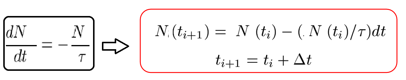
We should use  a discrete time and obtain the corresponding N as a function of time, where \tau is a constant.

clear
dt=0.1;t(1)=0;
N(1) =100;tau =1;
for j=2:round(5/dt);
    N(j)=Nu(j-1)-N(j-1)/tau*dt;
    t(j)=t(j-1)+dt;
end

Here we can obtain more accurate results by reducing dt but the time cost will be increased. round is the function in Octave, returning an integer. To check whether the result is correct, we can plot the data of t and N. The exact solution is also plot for comparison.

plot(t,N,'o-')
hold on
plot(t,N(1)*exp(-t/tau),'r-*')

(3) Differential Equations (with second-order derivative)

Consider a falling object, we have the equation:

 

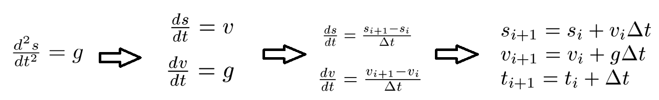
We change the  differential equation with second-order derivative into two differential equations with first-order derivative. Then, we can solve them with the iteration.

clear
g=9.8;dt=0.2;
t(1)=0;v(1)=0;s(1)=0;
for j=2:round(4/dt);
    s(j)=s(j-1)+v(j-1)*dt;
    v(j)=v(j-1)+g*dt;
    t(j)=t(j-1)+dt;
end