tensor flow

笔记：

图的定义和图的运行完全分开：
在tensorflow中，需要预先定义各种变量，建立相关的数据流图，在数据流图中创建各种变量之间的计算关系，完成图的定义，需要把运算的输入数据放进去后，才会形成输出值。

Tensor
张量，是tensorflow中最主要的数据结构，张量用于在计算图中进行数据传递，创建了张量后，需要将其赋值给一个变量或占位符，之后才会将该张量添加到计算图中。

实验：

import tensorflow as tf
from tensorflow import keras
import numpy as np
import matplotlib.pyplot as plt

print(tf.__version__)

fashion_mnist = keras.datasets.fashion_mnist

(train_images, train_labels), (test_images, test_labels) = fashion_mnist.load_data()

class_names = ['T-shirt/top', 'Trouser', 'Pullover', 'Dress', 'Coat',
'Sandal', 'Shirt', 'Sneaker', 'Bag', 'Ankle boot']

train_images.shape
len(train_labels)
train_labels
test_images.shape
len(test_labels)

plt.figure()
plt.imshow(train_images[0])
plt.colorbar()
plt.grid(False)
plt.show()

train_images = train_images / 255.0

test_images = test_images / 255.0

plt.figure(figsize=(10,10))
for i in range(25):
plt.subplot(5,5,i+1)
plt.xticks([])
plt.yticks([])
plt.grid(False)
plt.imshow(train_images[i], cmap=plt.cm.binary)
plt.xlabel(class_names[train_labels[i]])
plt.show()

model = keras.Sequential([
keras.layers.Flatten(input_shape=(28, 28)),
keras.layers.Dense(128, activation='relu'),
keras.layers.Dense(10)
])

model.compile(optimizer='adam',
loss=tf.keras.losses.SparseCategoricalCrossentropy(from_logits=True),
metrics=['accuracy'])

model.fit(train_images, train_labels, epochs=10)

test_loss, test_acc = model.evaluate(test_images, test_labels, verbose=2)

print('\nTest accuracy:', test_acc)

probability_model = tf.keras.Sequential([model,
tf.keras.layers.Softmax()])
predictions = probability_model.predict(test_images)
predictions[0]
np.argmax(predictions[0])
test_labels[0]

def plot_image(i, predictions_array, true_label, img):
predictions_array, true_label, img = predictions_array, true_label[i], img[i]
plt.grid(False)
plt.xticks([])
plt.yticks([])

plt.imshow(img, cmap=plt.cm.binary)

predicted_label = np.argmax(predictions_array)
if predicted_label == true_label:
color = 'blue'
else:
color = 'red'

plt.xlabel("{} {:2.0f}% ({})".format(class_names[predicted_label],
100*np.max(predictions_array),
class_names[true_label]),
color=color)

def plot_value_array(i, predictions_array, true_label):
predictions_array, true_label = predictions_array, true_label[i]
plt.grid(False)
plt.xticks(range(10))
plt.yticks([])
thisplot = plt.bar(range(10), predictions_array, color="#777777")
plt.ylim([0, 1])
predicted_label = np.argmax(predictions_array)

thisplot[predicted_label].set_color('red')
thisplot[true_label].set_color('blue')

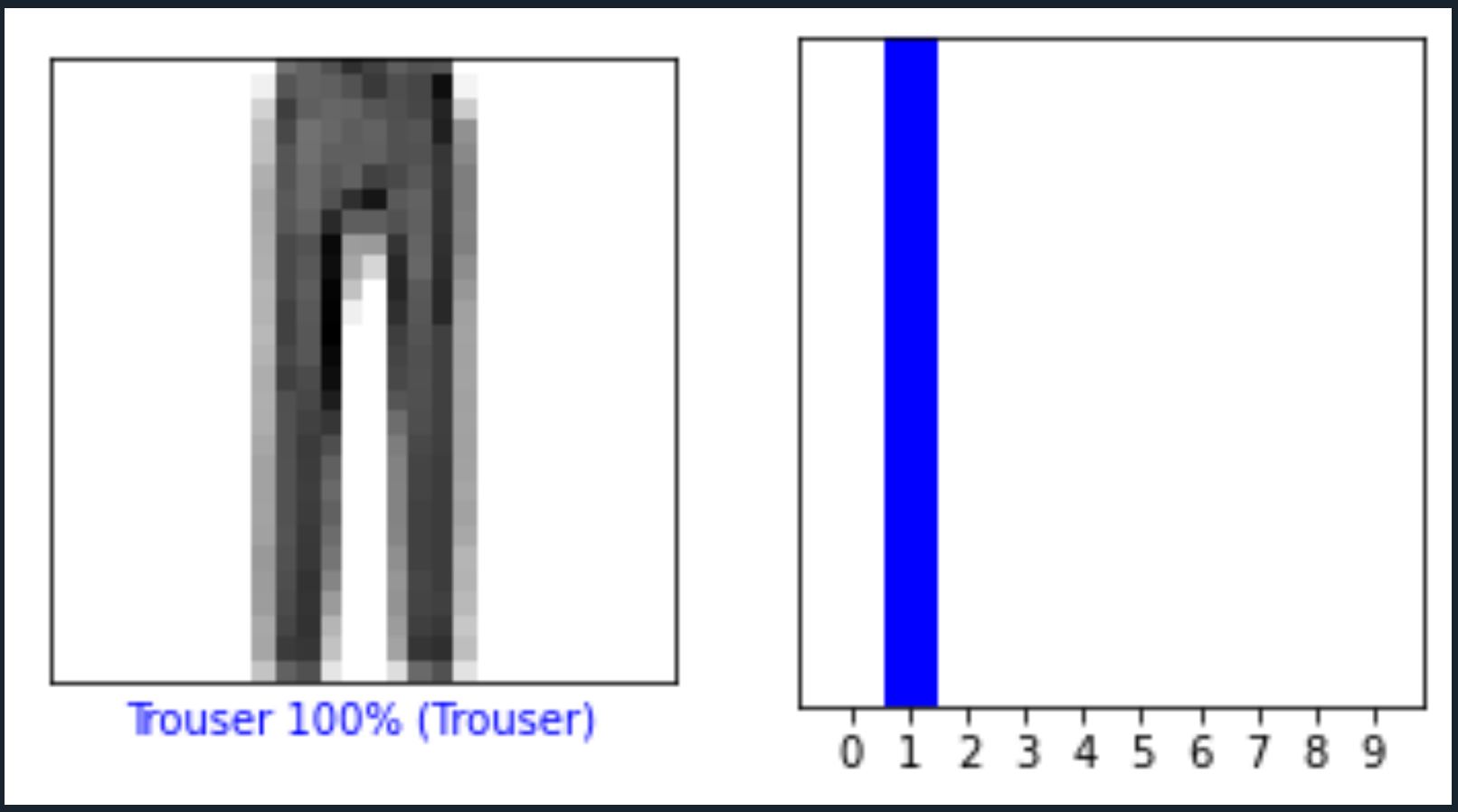
i = 0
plt.figure(figsize=(6,3))
plt.subplot(1,2,1)
plot_image(i, predictions[i], test_labels, test_images)
plt.subplot(1,2,2)
plot_value_array(i, predictions[i], test_labels)
plt.show()

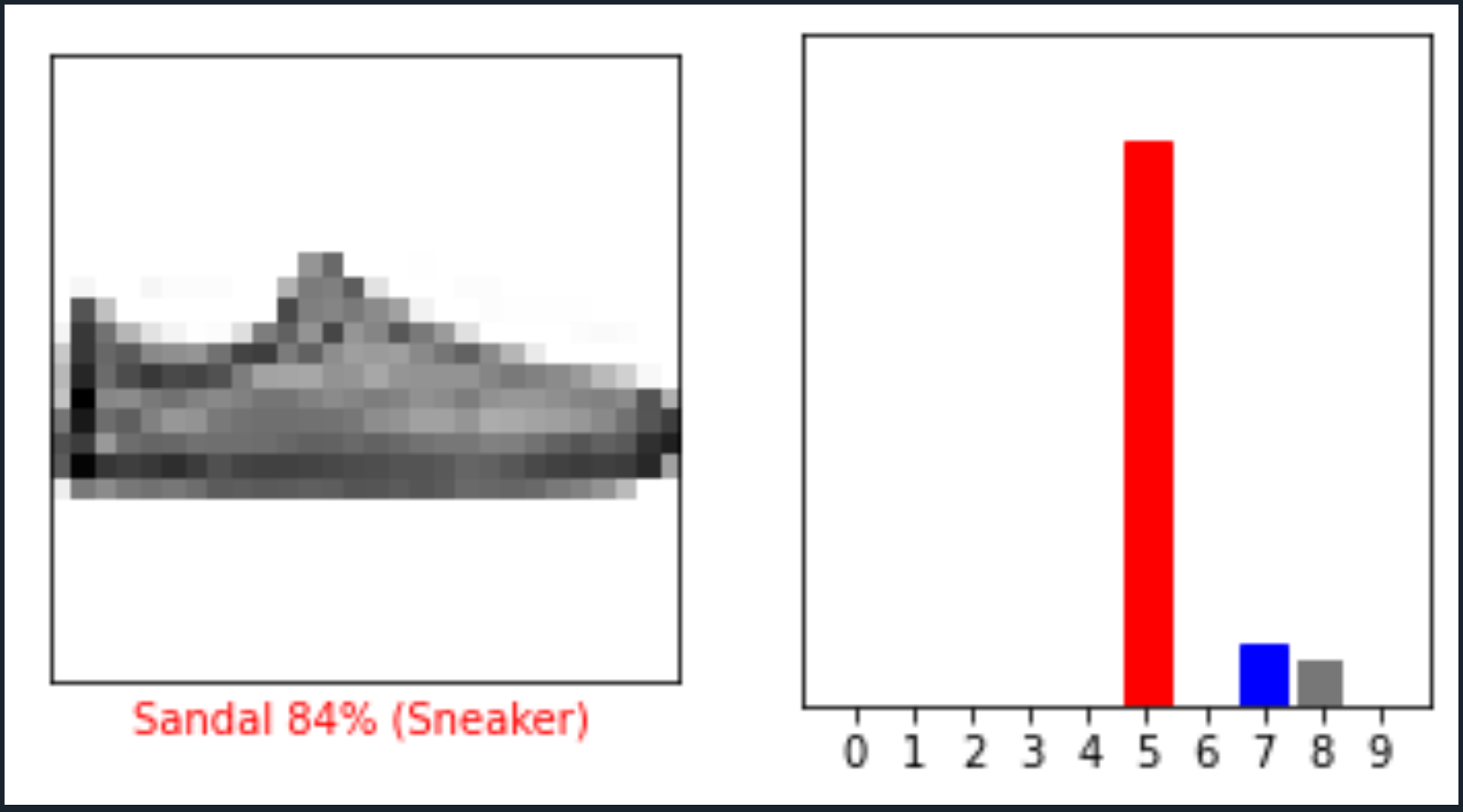
i = 12
plt.figure(figsize=(6,3))
plt.subplot(1,2,1)
plot_image(i, predictions[i], test_labels, test_images)
plt.subplot(1,2,2)
plot_value_array(i, predictions[i], test_labels)
plt.show()

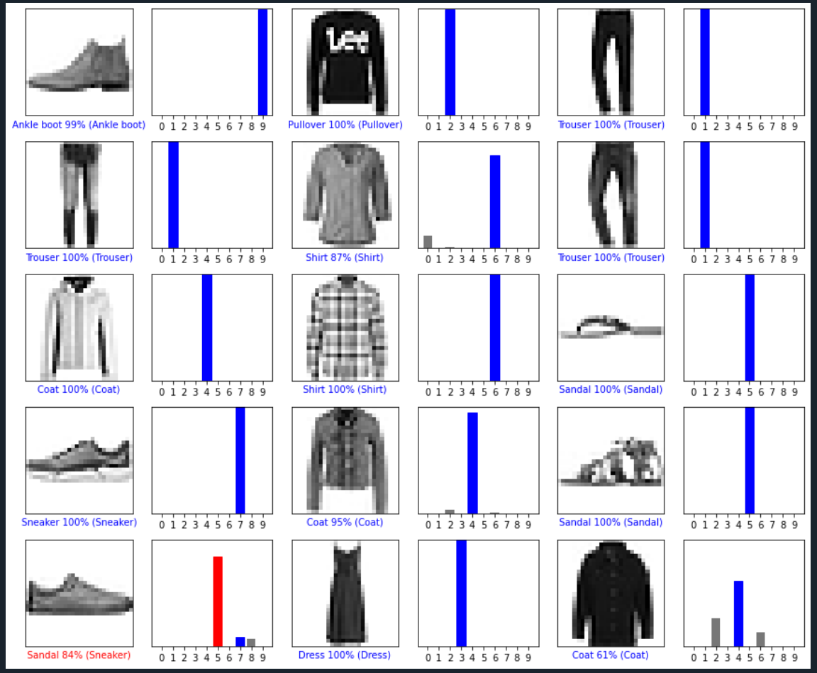
num_rows = 5
num_cols = 3
num_images = num_rows*num_cols
plt.figure(figsize=(2*2*num_cols, 2*num_rows))
for i in range(num_images):
plt.subplot(num_rows, 2*num_cols, 2*i+1)
plot_image(i, predictions[i], test_labels, test_images)
plt.subplot(num_rows, 2*num_cols, 2*i+2)
plot_value_array(i, predictions[i], test_labels)
plt.tight_layout()
plt.show()

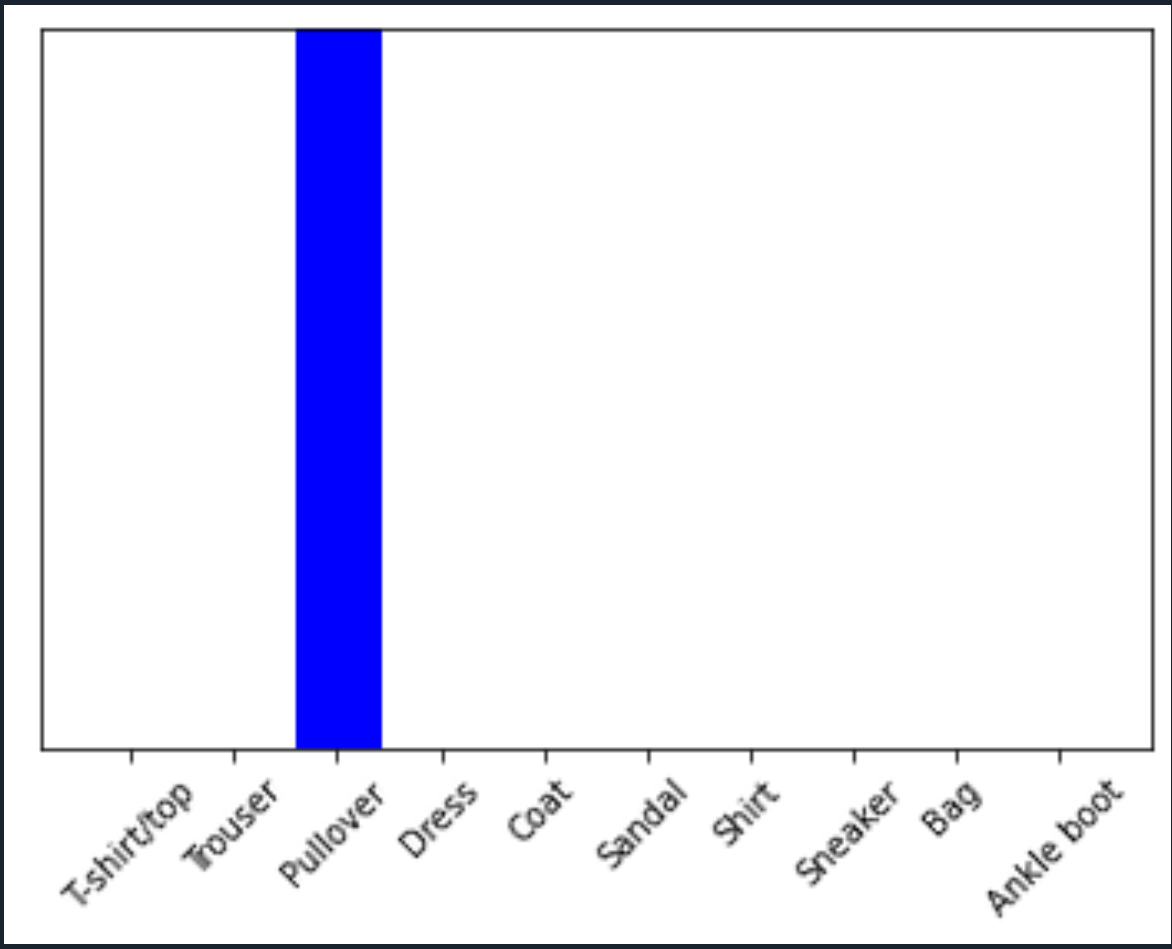
img = test_images[1]

print(img.shape)

img = (np.expand_dims(img,0))

print(img.shape)

predictions_single = probability_model.predict(img)

print(predictions_single)

plot_value_array(1, predictions_single[0], test_labels)
_ = plt.xticks(range(10), class_names, rotation=45)

np.argmax(predictions_single[0])

结果：