

机器学习、深度学习总结
机器学习、深度学习总结
目前包括:
输入归一化、参数初始化、批归一化、Dropout、全连接层、激励函数、卷积层、池层、ResNet 、Inception网络、损失函数、正则化、多分类、梯度下降、SVM等
输入归一化
- 为了减少迭代的次数,使用输入归一化,将输入改写成均值为0,范围一致的分布形式。
tf.image.per_image_standardization(image)
#image:An n-D Tensor with at least 3 dimensions, the last 3 of which are the dimensions of each image.
def per_image_standardization(image):
  """Linearly scales each image in `image` to have mean 0 and variance 1.
  For each 3-D image `x` in `image`, computes `(x - mean) / adjusted_stddev`,
  where
  - `mean` is the average of all values in `x`
  - `adjusted_stddev = max(stddev, 1.0/sqrt(N))` is capped away from 0 to
    protect against division by 0 when handling uniform images
    - `N` is the number of elements in `x`
    - `stddev` is the standard deviation of all values in `x`
  Args:
    image: An n-D Tensor with at least 3 dimensions, the last 3 of which are the
      dimensions of each image.
  Returns:
    A `Tensor` with same shape and dtype as `image`.
  Raises:
    ValueError: if the shape of 'image' is incompatible with this function.
  """
  with ops.name_scope(None, 'per_image_standardization', [image]) as scope:
    image = ops.convert_to_tensor(image, name='image')
    image = _AssertAtLeast3DImage(image)

    # Remember original dtype to so we can convert back if needed
    orig_dtype = image.dtype
    if orig_dtype not in [dtypes.float16, dtypes.float32]:
      image = convert_image_dtype(image, dtypes.float32)

    num_pixels = math_ops.reduce_prod(array_ops.shape(image)[-3:])
    image_mean = math_ops.reduce_mean(image, axis=[-1, -2, -3], keepdims=True)

    # Apply a minimum normalization that protects us against uniform images.
    stddev = math_ops.reduce_std(image, axis=[-1, -2, -3], keepdims=True)
    min_stddev = math_ops.rsqrt(math_ops.cast(num_pixels, image.dtype))
    adjusted_stddev = math_ops.maximum(stddev, min_stddev)

    image -= image_mean
    image = math_ops.div(image, adjusted_stddev, name=scope)
    return convert_image_dtype(image, orig_dtype, saturate=True)
参数初始化
- 0初始化:
- 所谓0初始化就是将所有的参数都初始化为零,但是由于初始化的值是一样的,它将不能破坏对称,以至于所有同源的参数的值将永远一样。
- 具有相同激活函数的两个隐藏单元连接到相同单元,那么这些单元必须具有不同的初始参数。一旦他们具有相同的初始参数,然后应用到确定性损失和模型的确定性学习算法将一直以相同的方式更新这两个
- 随机初始化:
- 梯度爆炸: \(W>I\)
- 梯度消失:\(W<I\)
- Xavier初始化:根据前向传播公式\(z = \sum w_i x_i\)且\(w\)与\(x\)独立分布,我们可以求出方差\(Var(z) = n_xVar(w_i)Var(x_i)\), 如果我们希望\(Var(z) = Var(x)\),那么需要使\(n_xVar(w) = 1\)即,\(Var(w) = \frac{1}{n_x}\);在反向传播中\(dA^{[l-1]} = W^{[l]T}dZ^{[l]}\),设激励函数为线性且导数为1,那么\(Var(dz^{[l-1]}) = n_l Var(w) Var(dz^{[l]})\)。因此我们可以看出,在前向传播中,我们希望\(Var(w) = \frac{1}{n_{l-1}}\),在反向传播中我们希望\(Var(w) = \frac{1}{n_{l}}\)因此,在Xavier初始化中,我们令\(Var(w) = \frac{2}{n_{l-1} + n_l}\),即在均分分布(\(Var = \frac{(b-a)^2}{12}\))中
- W = 1的参数初始化还有什么?
批归一化(Batch Normalization-BN)
在隐藏层中的优化
- 在TensorFlow的实现:计算:\(\frac{\gamma(x-\mu)}{\sigma}+\beta\)
tf.nn.batch_normalization(
    x, mean, variance, offset, scale, variance_epsilon, name=None
)
其中mean和variance由函数tf.nn.moments(..., keepdims=False)得到,这也是tf里计算mean和variance的函数。
- BN global(除了输入限制为4D没发现什么重要的区别)
- BN keras(还没看懂)
Dropout
Dropout是正则化的一种方式,由名字退出(drop out)可以看出,它是以随机除去神经元来使得减少某个神经元的依赖程度,达到可以使用正则化的方式。在应用过程中,我们设置一个新的变量\(D^{[l]}=[d^{[l](1)}...d^{[l](m)}]\)用以表示第l个隐藏层的D,其中每一个d(i)表示在第i个数据下的d,而d表示的是该神经元是否隐藏。因此它将是一个由0和1组成的向量。使用\(d^{[l](i)}=np.random.rand(a^{[l](i)}.shape)<keep\_prob\)来设置d和D。之后为了使得输出结构的均值保持不变,在使用了Dropout的隐藏层在正向传播求得\(A^{[ l ]}\) 之后还要再除以\(keep\_prob\)。并且在反向传播时也要将\(dA = \frac{dA}{keep\_prob}\)
全连接层
- 前项传播
卷积层
层数公式:
1x1卷积层: 可以降维或者升维,一般用于减少参数
- 空间卷积、反卷积、转置卷积?
Pool层
分为average pooling和max pooling
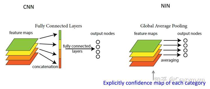 Fig. FC vs GAP
tf.keras.layers.GlobalAveragePooling2D(
    data_format=None, **kwargs
)
 Fig. FC vs GAP vs GMP
参考:
ResNet Model
由于在神经网络很深的时候,会出现性能翻转的问题,即随着层数的增加,training error反而会增大(degradation problem),因此引用了ResNet。假设在一种网络A的后面添加几层形成新的网络B,如果增加的层级只是对A的输出做了个恒等映射(identity mapping),即A的输出经过新增的层级变成B的输出后没有发生变化,这样网络A和网络B的错误率就是相等的,也就证明了加深后的网络不会比加深前的网络效果差。
- 在TensorFlow中的实现:
 Fig. Resnet(v1) vs resnet(v2)
Resnet(v1)的特点是几个块,除第一个块内第一层stride=1,其它块内第一层stride=2,每深一块深度\(\times 2\),并使用相同stride的1x1卷积层将输入也改变为同深度的tensor。块内的卷积层相同,切没个两层有一个shotcut用以实现ResNet。本例每个块内有\(3 \times 2 = 6\)层,一共有\(3 \times 3 \times 2 + 2 = 20\)层
    for stack in range(3):#number of stack, each stack contain 6 layers
        for res_block in range(num_res_blocks):
            strides = 1
            #can be seen in the resual block, the first layer(except the first stack) stride = 2
            if stack > 0 and res_block == 0:  # first layer but not first stack
                strides = 2  # downsample
            y = resnet_layer(inputs=x,
                             num_filters=num_filters,
                             strides=strides)
            #why there is an additional y here?,because we need to add the shotcut term, and notice that we donot use strides here
            y = resnet_layer(inputs=y,
                             num_filters=num_filters,
                             activation=None)
            if stack > 0 and res_block == 0:  # first layer but not first stack
                # linear projection residual shortcut connection to match
                # changed dims
                x = resnet_layer(inputs=x,
                                 num_filters=num_filters,
                                 kernel_size=1,
                                 strides=strides,
                                 activation=None,
                                 batch_normalization=False)
            x = tensorflow.keras.layers.add([x, y])
            x = Activation('relu')(x)
        num_filters *= 2
Resnet(v2):第一个捷径使用Conv2D(1), 之后的不经过卷积层。每个阶段开始,feature map将被步长为的卷积层减半,filters的数量增倍,在每个阶段中,每个卷积层有相同数目的filters和filters size。即:
- Conv1:(32,32);16
- Stage 0:(32,32);64
- Stage 1:(16,16);128
- Stage 2:(8,8);256
    for stage in range(3):
        for res_block in range(num_res_blocks):
            activation = 'relu'
            batch_normalization = True
            strides = 1
            if stage == 0:#first stage(block)
                num_filters_out = num_filters_in * 4
                if res_block == 0:  # first layer and first stage
                    activation = None
                    batch_normalization = False
            else:
                num_filters_out = num_filters_in * 2
                if res_block == 0:  # first layer but not first stage
                    strides = 2    # downsample

            # bottleneck residual unit
            y = resnet_layer(inputs=x,
                             num_filters=num_filters_in,
                             kernel_size=1,
                             strides=strides,
                             activation=activation,
                             batch_normalization=batch_normalization,
                             conv_first=False)
            y = resnet_layer(inputs=y,
                             num_filters=num_filters_in,
                             conv_first=False)
            y = resnet_layer(inputs=y,
                             num_filters=num_filters_out,
                             kernel_size=1,
                             conv_first=False)
            if res_block == 0:
                # linear projection residual shortcut connection to match
                # changed dims
                x = resnet_layer(inputs=x,
                                 num_filters=num_filters_out,
                                 kernel_size=1,
                                 strides=strides,
                                 activation=None,
                                 batch_normalization=False)
            x = tensorflow.keras.layers.add([x, y])

        num_filters_in = num_filters_out
Inception网络
使用多个相同长宽(可能不同深度)进行叠加,形成Inception网络。
-和ResNet的联系,实战?
损失函数
机器学习分为监督学习和无监督学习,他们之间的区别在于监督学习有数据和真实值,即X,Y;而监督学习只有数据,没有真实值,即X。其中监督学习分为线性回归和分类,而无监督学习只有分类。
线性回归主要是做预测,即使用数据集和真实值(以后已训练集来代替)用线性拟合来形成一条曲线。主要使用的损失函数式MSE(均方误差),即:
损失函数问题:而为什么在线性回归中使用MSE而在逻辑回归中使用交叉熵作为损失函数:
- 从MSE和交叉熵的目的来说,MSE表示真值与预测值之间的距离;交叉熵表示预测概率分布与真实概率分布的问题,对于分类来说使用概率分布更加的合理。且对于线性回归问题有负数,log(-1.5)无法计算
- 在分类问题中,开始会使用Sigmoid函数作为激励函数,而如果将sigmoid函数带入到交叉熵之中的时候,会产生非凸函数,即有多个极点的函数,这是梯度下降所无法解决的问题。
激励函数
激励函数问题:sigmoid, Tanh, Relu的区别:
 Fig. 1 sigmoid, tanh, relu
Tanh函数:\(tanh(x) = \frac{e^x - e^{-x}}{e^x + e^{-x}}\)
特点:比起sigmoid来说优点是其中心对称
缺点:还是有软饱和问题;exp计算量大的问题
Relu函数:\(max(0,x)\)
特点:正数不饱和,负数硬饱和;比sigmoid和tanh比计算量小
缺点:非中心对称
正则化
正则化:在使用损失函数构建成本函数的时候有一项很重要的就是正则化。一般来说正则化分为两种:L1正则化和L2正则化
- L1正则化:\(J_{\theta R_1} = J_{\theta} + \lambda \sum \|\theta_j\|\)
- L2正则化:\(J_{\theta R_2} = J_{\theta} + \lambda \sum \theta_j^2\)
- L1正则化目的是使参数更加稀疏,通俗来讲是是参数为0的项更多;L2正则化目的是减少参数的权重
二分类与多分类
输出之前
在说到逻辑回归问题时,它有二分类问题和多分类问题,那么他们的区别和联系是:
- 一般使用sigmoid来处理二分类问题:\(\delta(x) = \frac{1}{1+e^{-x}}\)
- 使用softmax函数来处理多分类问题:\(S(x_j) = \frac{e^{x_j}}{\sum^K_{k=1} e^{x_k}}\), j = 1 ... K
梯度下降
梯度下降:梯度下降是求解机器学习/深度学习问题的基础但是由于批梯度下降处理速度慢、计算量下降因此引入了mini-batch梯度下降之后出现了收敛震荡的问题,引出以下三种方法用以做梯度下降的加速。
- Momentum:使用指数权重平均,为dw和db做平均
SVM
SVM(support vecter machine)支持向量机:SVM是从逻辑回归变化而来的,由于逻辑回归的损失函数为:

 浙公网安备 33010602011771号