人工智能实战 第3次作业 郑浩

项目	内容
这个作业属于哪个课程	人工智能实战 2019（北京航空航天大学）
这个作业的要求在哪里	第三次作业：使用minibatch的方式进行梯度下降
我在这个课程的目标是	了解人工智能的基础理论知识，锻炼实践能力
这个作业在哪个具体方面帮助我实现目标	学习梯度下降的原理和几种算法，并通过代码实践来练习
作业正文	见下文
其他参考文献	无

1.作业要求

• 使用minibatch的方式进行梯度下降
• 采用随机选取数据的方式
• 复习讲过的课程（链接），并回答关于损失函数的 2D 示意图的问题：
  问题2：为什么是椭圆而不是圆？如何把这个图变成一个圆？
  问题3：为什么中心是个椭圆区域而不是一个点？

2.解题思路

见课堂课件内容

3.代码

import numpy as np
import matplotlib.pyplot as plt
from pathlib import Path

x_data_name="TemperatureControlXData.dat"
y_data_name="TemperatureControlYData.dat"

def ReadData():
    Xfile=Path(x_data_name)
    Yfile=Path(y_data_name)
    if Xfile.exists() & Yfile.exists():
        X=np.load(Xfile)
        Y=np.load(Yfile)
        return X.reshape(1,-1),Y.reshape(1,-1)
    else:
        return None,None

def GetBatchSamples(X,Y,batch_size,max_iter,r_index):
    X_batch=[]
    Y_batch=[]
    for i in range(0,max_iter):
        index=r_index[i*batch_size:(i+1)*batch_size]
        X_batch.append(X[0][index].reshape(1,batch_size))
        Y_batch.append(Y[0][index].reshape(1,batch_size))
        
    return X_batch,Y_batch

def ForwardCalculationBatch(w,b,batch_x):
    z=np.dot(w,batch_x)+b
    return z

def BackPropagationBatch(x,y,z):
    k=x.shape[1]
    dz=z-y
    dw=np.dot(dz,x.T)/k
    db=np.dot(dz,np.ones(k).reshape(batch_size,1))/k
    return dw, db

def UpdateWeights(w,b,dw,db,eta):
    w=w-eta*dw
    b=b-eta*db
    return w,b

def CheckLoss(w,b,x,y):
    k=x.shape[1]
    z=np.dot(w,x)+b
    LOSS=(z-y)**2
    loss=LOSS.sum()/k/2
    return loss

def random_index(n):
    test=np.arange(n)
    np.random.shuffle(test)
    return test

if __name__ == '__main__': 
    X, Y=ReadData()
    num_example=X.shape[1]
    num_feature=X.shape[0]
    eta=0.01
    batch_range=[5,10,15]
    batch_result={}
    
    for batch_size in batch_range:
        max_epoch=50
        max_iter=int(num_example/batch_size)
        w,b=0,0
        loss_result=[]
        for epoch in range(max_epoch):
            r_index=random_index(num_example)
            X_batch,Y_batch=GetBatchSamples(X,Y,batch_size,max_iter,r_index)
            for iteration in range(0,max_iter):
                x=X_batch[iteration]
                y=Y_batch[iteration]
                z=ForwardCalculationBatch(w,b,x)
                dw,db=BackPropagationBatch(x,y,z)
                w,b=UpdateWeights(w,b,dw,db,eta)
                erro=CheckLoss(w,b,X,Y)
                loss_result.append(erro)
        batch_result[str(batch_size)]=loss_result

    plt.figure(figsize=(16, 10))
    p5,=plt.plot(batch_result['5'])
    p10,=plt.plot(batch_result['10'])
    p15,=plt.plot(batch_result['15'])
    plt.legend([p5,p10,p15],["batch_size=5","batch_size=10","batch_size=15"])
    plt.ylim(0.006,0.1)
    plt.xlim(0,800)
    plt.xlabel('epoch')
    plt.ylabel('loss')
    plt.title("Learning Rate "+str(eta))
    plt.show()

4.实验结果

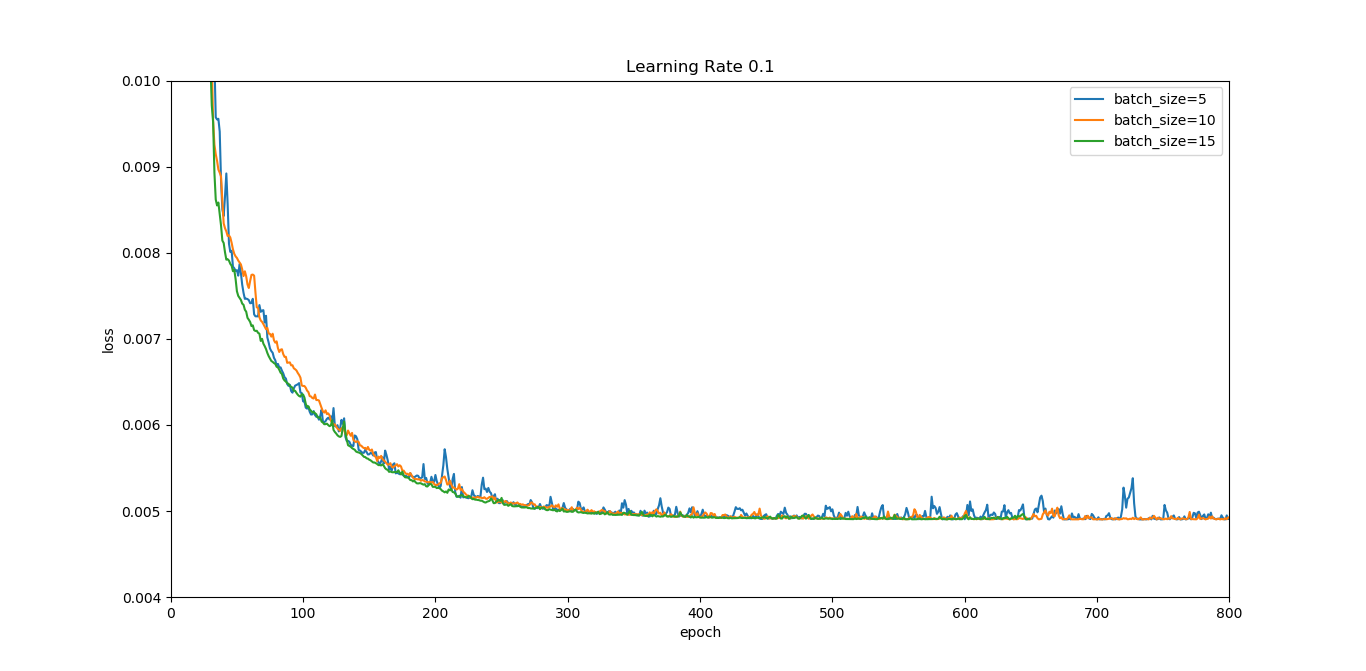
• 当eta=0.1时
  

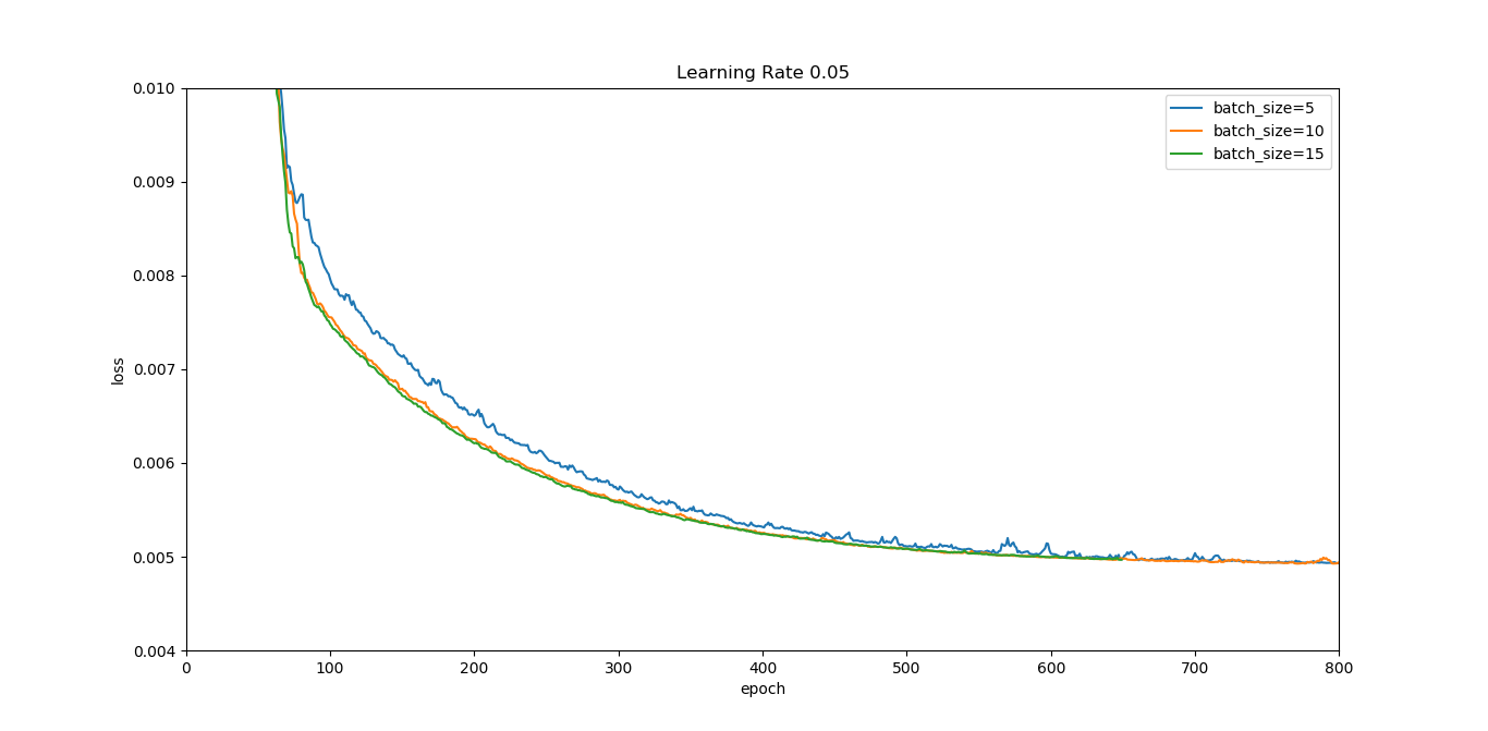
• 当eta=0.05时
  

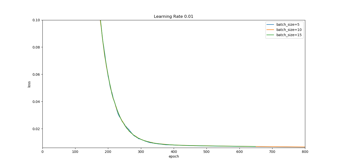
• 当eta=0.01时
  

5.实验结论

可以看到，eta越小，均方差损失loss的波动程度越小。同时，在eta一定的情况下，batch_size越大，loss的波动程度也越小。

6.额外问题

• 问题2：为什么是椭圆而不是圆？如何把这个图变成一个圆？
  　答：损失函数\(Loss=\frac{1}{2m}\sum_{i=1}^{m}{(x_iw+b-y_i)^2}\)
  \(=\sum_{i=1}^{m}{(x_i^2w^2+b^2+2x_ibw-2y_ib-2x_iy_iw+y_i^2)}\)
  可得，损失函数为椭圆函数。
  因此，当\(\sum_{i=1}^{m}{x_i^2}=1\)时，椭圆函数退化为圆。

• 为什么中心是个椭圆区域而不是一个点？
  答：理论上loss的最小值是一个点，但是计算机的计算是离散的，颜色相同的区域由于loss非常接近，于是被计算机视为是loss相同的点。